After discussing DP as DAGs, Shortest path on DAGs & LIS in O(nlogn), Levenshtein Edit Distance & Chain Matrix Multiplication we are finally here.

The Knapsack Problem

The Knapsack is probably one of the most famous problems used to introduce Dynamic Programming to new learners. It asks the following question, “Given a list of $n$ elements, each of which have some value $v_i$ and weight $w_i$ associated with them, what is the maximum value of elements I can fit into my Knapsack given that my Knapsack can only hold at max a weight of $W$ capacity?”

There are two variations of the above problem as well. The simpler one assumes that we have an infinite quantity of each element. That is, we can pick an element as many times as we wish. The harder version does not assume this. Each element can only be picked once.

A toy example

For the sake of illustration, we’ll assume we are attempting to solve the Knapsack for the given inputs

knapsack-1

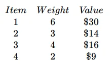
We have 4 items with their respective $v_i$ and $w_i$ values. Our Knapsack has a maximum capacity of $W = 10$.

With repetition

If repetition is allowed, we can solve the problem using a very simple approach. All we need to observe is that to compute the maximum value for a bag of capacity $W$, we can simply brute force over all elements with a simple recurrence.

Let $F(W)$ be the maximum value obtainable for a bag of capacity $W$. Then,

$$ \begin{aligned} F(W) = max(v_1+F(W-w_1), \ \dots \, v_n+F(W-w_n)) \\ \text{In our example, this corresponds to the following computation } \implies \\ F(10) = max(30+F(10-6), 14+F(10-3), 16+F(10-4), 9+F(10-2)) \\ \implies F(10) = max(30 + F(4), 14+F(7), 16+F(6), 9+F(8)) \end{aligned} $$

The idea behind this recurrence is as follows. At any capacity $W$, we are simply picking every possible element and asking what is the maximum value I can achieve after picking each element. It’s more or less just a brute force that considers picking every element for each capacity $W$.

It is easy to see that we are computing the answer for $W$ such sub-problems from $W_i = 1 \to W$. And at each sub-problem, we are iterating over $n$ elements.

It is also important to note that we do not consider including the element in our brute force when we reach a state where $W-w_i \lt 0$. This is an impossible/unreachable state. The base case is when we no longer have any elements which we can fit into the bag.

Hence we have $W$ sub-problems.
We are doing $O(n)$ computation at every node.
The recurrence is as described above.
The DAG structure is also easy to reason about. It’s simply just a linear chain from state
$W_i = 1 \to 2 \to \dots \to W$
Therefore, our final algorithm will have $O(nW)$ complexity.

Further, since there are only $O(W)$ subproblems, we only need $O(W)$ space to store the DP table.

Without repetition

Notice that our previous solution will not work here. Because we cannot choose elements multiple times. However, the order of choosing the elements does not matter either. But because of this condition, notice that it is not enough to simply consider subproblems defined by just one characteristic.

That is, a subproblem in the previous case was simply identified by $W$, the size of the Knapsack. Here, this is no longer the case. A “state” or “subproblem” has at least two changing variables. Both the number of elements we are including into the Knapsack and the weight of the Knapsack.

The new DP state

That is, we must change the definition of our DP to a 2-d DP where $DP[i][j]$ represents the state where we are considering the first $i$ elements among the list of available elements and our Knapsack is of size $j$.

Number of subproblems
Since we have $n$ possible prefixes which we will consider and $W$ possible values for the weight, we have of the order $O(nW)$ subproblems to compute
Finding the solution at some node
Notice that since we changed the definition of our DP to storing the best possible answer to the problem given that our Knapsack has size $W$ and we are only considering the first $i$ elements, when computing $DP[i][j]$, notice that we are only trying to include the $i^{th}$ element wherever it maximizes our answer.
This has the important implication that we do not need to brute force over $n$ elements at some state $[i, j]$. We only need to check the states $[i-1, W-w_i]$. This is $O(1)$ computation at every node.
Coming up with the recurrence
We are essentially trying to answer the question
“At some capacity $W$, when considering the $i^{th}$ element, does including it in the Knapsack help increase the previously obtained score at capacity $W$ when considering only $i-1$ elements?”
Writing this recurrence formally,
$F(i, W) = max \{ F(i-1, W), F(i-1, W-w_i) \}$
The first term in the max represents the previously obtained score at capacity $W$. The second term is the value we would get if we tried including element $i$ when considering a bag of size $W$.
The DAG structure for this problem is very similar to the structure obtained when solving the Edit distance problem. It is simply a graph where each state $[i, W]$ depends on the state $[i-1, W-w_i]$.
We have an algorithm that requires us to perform $O(1)$ computation for each of the $O(nW)$ subproblems. Hence the total running time will be $O(nW)$. However, since there are $nW$ subproblems, we will also require $O(nW)$ space.

Can we do better?

This time, we actually can! Notice that just like how we did in the Edit distance problem, the DP state at any $[i, W]$ is ONLY dependent on the DP states exactly one level below it. That is, every DP value in row $i$ is only dependent on the DP values in row $i-1$.

This means that again, we can do the exact same thing and use Single Row Optimization to reduce the space complexity of our DP from $O(nW)$ to just $O(W)$. For small values of $W$, we might even consider this linear!

Pseudo-polynomial-time algorithms

At first glance, it is very easy to write off the Knapsack problem as belonging to the $P$ complexity class (Introduction to Complexity Theory). After all, it seems to just be quadratic right?

But this is not true. We define the complexity of algorithms based on input size $n$.

To be more precise: Time complexity measures the time that an algorithm takes as a function of the length in bits of its input.

However, notice that in this case, the complexity of our algorithm relies on both $n$ and $W$. $W$ is the value of an input. If we consider $W$ in binary, we would require $log_2(W)$ bits to represent $W$. If the input is in binary, the algorithm becomes exponential.

Why?

We will try to explain this by means of a nice example.

Let’s say we are trying to solve the problem for $n = 3$ and $W = 8$. Keep in mind that $W = 1000$ in binary. That is, $W$ is 4 bits long.
Hence total complexity = $O(nW) \implies O(3 \times 8) = O(24)$
Now let’s increase $n$ to $n = 6$. We have linearly multiplied it by $2$. Notice that this still gives us
Time complexity: $O(nW) \implies O(6 \times 8) = O(48)$. It is the expected increase by 2.
Now let us increase $W$ by a factor of 2. Notice that this means we double the length of W in bits. Not the value of W itself. This means $W$ will now be represented by $W = 8$ bits. This means $W$ is now equal to $10000000$ in binary.
This gives us a complexity of $O(nW) \implies O(3 \times 2^8) = O(768)$. That is, there is an exponential increase in complexity for a linear increase in $W$ .

Knapsack is NP-Complete

The Knapsack problem is in fact, an NP-Complete problem. There exists no known polynomial-time algorithm for this problem. However, it is nice to know that is it often classes as “Weakly np-complete.”

That is, for small values of $W$we can indeed solve the optimization problem in polynomial time. If we give input $W$ in the form of smaller integers, it is weakly NP-Complete. But if the value $W$ is given as rational numbers, it is no longer the case.

Alternate Version of the Knapsack problem

While we solved the Knapsack problem in the standard manner by defining $DP[i][j]$ as the maximum value achievable when considering the first $i$ elements and a bag of capacity $j$, what do we do if the value of $W$ is large, but the value of $\sum_{i}^{n}v_i$ is small?

Consider the following two problems from the AtCoder Educational DP contest.

Knapsack - 1

The first problem is simply the standard Knapsack problem.

The constraints for it were as follows,

$$ \begin{aligned} 1 \leq N \leq 100 \\ 1 \leq W \leq 10^5 \\ 1 \leq w_i \leq W \\ 1 \leq v_i \leq 10^9 \end{aligned} $$

A $O(nW)$ solution would take around $1e7$ operations which should pass comfortably.

Here’s a link to my submission: Submission Link

Knapsack - 2

The second problem is a little different. It asks the same question, but for different constraints.

$$ \begin{aligned} 1 \leq N \leq 100 \\ 1 \leq W \leq 10^9 \\ 1 \leq w_i \leq W \\ 1 \leq v_i \leq 10^3 \end{aligned} $$

Notice that $W$ is now $10^9$. $O(nW)$ would now take 1e11 operations. This would practically have a very slow running time in comparison to our previous ~1e7 operation solution.

We will have to think of something different.

Notice that for this problem, the values $v_i$ are much smaller. In fact, considering $n=100$ elements, the maximum value obtainable is just $max(v_i)\times n = 10^5$.

Now, we can exploit this by doing the same Knapsack DP, but this time, instead of storing the maximum value achievable in max capacity $j$ when considering the first $i$ elements, we redefine the dp as follows.

$DP[i][j]$ will now store the minimum weight required to achieve value $j$ when considering just the first $i$ elements. We can now simply pick the maximum $j$ in row $i=n$ which satisfies the condition $DP[i][j] \leq W$.

This solution runs in $O(n \times \sum_{i}^{n}v_i)$ which gives us $\approx1e5$ operations. This is much faster than the standard approach.