Activity Selection & Huffman Encoding
Interactive Graph
Table of Contents
Greedy Algorithms
As discussed previously, greedy algorithms are an amazing choice when we can prove that they do indeed give the optimal solution to some given problem. This signifies the importance of being able to prove the optimality of greedy solutions. In general, if the following two conditions hold, we can certainly say that a greedy strategy will give us the globally optimal answer.
Locally optimum choice
Given some problems, can we focus on its local state and solve for a solution that produces the most locally optimal solution at that state? In other words, we should be able to take one step towards the optimum solution.
Optimum substructure property
Once this step is taken, even after the change in state after taking that step, are we able to restate the problem such that the new problem is the same as the original problem, albeit for a smaller input?
Notice that if the answer to the above two questions is yes, then it is possible to prove that repeatedly taking the locally optimal choice will indeed give us the optimal solution. This is easily proven via induction.
Take the optimal step at any given step $i$, now restate the problem as a smaller version of the original problem, and again take the locally optimal step at $i+1$. We can inductively repeat till this is the final state where we can again take the optimal choice. Since we can solve each subproblem independently simply by taking the best choice at each step, the solution must be optimal.
Activity Selection
Consider the famous activity selection problem. The problem is as follows,
Given a set of activities $S=\{a_1, a_2,\dots,a_n\}$, where activity $a_i$ takes time $[s_i, f_i)$ to finish. Find the maximum number of activities that can be picked such that there are zero overlaps, i.e., pick the subset of the maximum size where all activities are disjoint.
The naïve solution would be to brute force over all $n!$ different permutations in linear time to find the optimal answer. This is obviously far too slow to be of much use to us. So, how can we do better? Would a greedy solution work?
Greedy #1
Sort the intervals by duration $|f_i-s_i|$ and greedily pick the shortest ones
Does this satisfy our two properties? The answer is… no. Notice that by picking the shortest interval activity, we cannot restate the problem for a smaller input the same way. We do not have optimum substructure. Consider the below case.
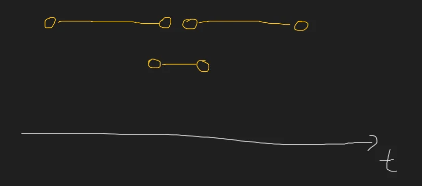
Greedily we would pick the middle activity, but this removes two activities for the next step. This problem has no optimum substructure. The optimal solution would be to pick both the large intervals.
Greedy #2
Greedily pick the activities that start the earliest
That approach follows neither property. Consider this case,
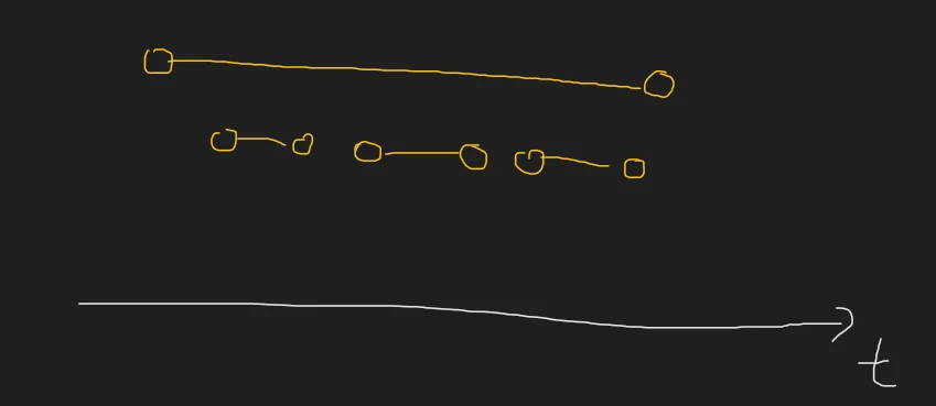
We are neither picking a locally optimum choice nor maintaining an optimum substructure. The greedy solution gives 1 whereas the answer is clearly, 3.
Greedy #3
Greedily pick the activities that end the earliest
Does this approach satisfy both criteria? The answer is… yes.
Let us pick the activity that ends the earliest. If this is not part of the optimal solution and the activity it overlaps with is part of the optimal solution, notice that because the activity we picked ends earlier, our activity cannot have any other overlap. Both contribute +1 to the solution and hence our activity is locally optimal. Further, since we have picked the earliest ending activity (which is optimal) we can cross off overlaps and restate the problem for smaller input. This approach maintains both properties! It must be right.
A more formal proof
Let us suppose that we know the answer. Let the answer be $A$. Let us sort $A$ by finish time such that $\forall a_{i Now, let our optimal choice activity be $x$. By virtue of our greedy choice, we know that $f_{x} \leq f_{a_i} \forall a_i \in A$ Consider $f_{a_0}$. If $x = a_0$, we are done. But if $x \neq a_0$, notice that $f_x \leq f_{a_0}$. This means that $x$ cannot overlap with any more activities in the set $A$ than $a_0$. And the set $A$ is disjoint by definition. Our solution can be written as Notice that $x$ cannot overlap with any element in $A$. This is because they’re the first choice to be picked, there is no overlap on the left. And $f_x \leq f_{a_0}$ implies there is no overlap on the right and both provide a $+1$ to the final answer. Hence $x$ must be an optimal choice. This solution is much better than our $O(n!)$ solution and can find the optimal answer in just $O(nlogn)$. The $nlogn$ comes from the sorting requirement. Let’s think about how computers store text. A lot of the text on machines is stored in ASCII. ASCII is a character encoding used by our computers to represent the alphabet, punctuations, numbers, escape sequence characters, etc. Each and every ASCII character takes up exactly one byte or 8 bits. The encoding chart can be found here Oftentimes, computers need to communicate with one another, and sending large volumes of text is not an uncommon occurrence. Communication over networks, however, have their own cost and speed disadvantages that make sending smaller chunks of data a very favorable option. This is one of the times when ranking an algorithm by space is preferred over ranking algorithms by time. As our metric for comparison between algorithms changes, so does our problem statement. “What is the most optimal way to losslessly compress data such that it takes up minimum space?” Notice that unlike video or audio compression, ASCII text compression must be lossless. If we lose any data, we have also lost the character. This means we can no longer figure out what the original ASCII character was. These requirements give us a few basic requirements that our algorithm must meet. The idea of compression is to reduce the size of the data being compressed. But ASCII requires 8 bytes. This means that we must try to encode data in fewer than 8 bytes based on the frequency of occurrence. This will allow us to dedicate fewer bits for more commonly occurring characters and more bits for characters that occur almost never, thus helping us compress our data. However, this implies that we need some form of variable-length encoding for our characters. One variable-length encoding that might work is the binary system. However, notice that the following assignment will fail. When we encounter the encoding $00$ in the compressed data, we no longer know whether it is “two spaces” or one “t” character. We have lost information in our attempt to compress data. This implies that our algorithm must fulfill the prefix-free property. That is while reading the compressed data, based on the prefix, we must be able to uniquely identify the character that it is representing. If this is not possible then we will not have an injective mapping and data will be lost. Back in the world of information theory, Shannon laid out the 4 key axioms regarding information. Information $I(x)$ and probability $P(x)$ are inversely related to each other Consider the following thought experiment. The second sentence conveys a lot more information than the first. The first statement is highly probable and hence does not convey as much information as the second. $I(x) \geq 0$ Observing an event never causes a loss in information $P(x)=1\implies I(x) = 0$ If an event is 100% certain to occur then there is no information to be gained from it $P(x\cap y)=P(x).P(y) \implies I(x\cap y)=I(x)+I(y)$ Two independent events if observed separately, give information equal to the sum of observing each one individually It can be proven that the only set of functions that satisfy the above criteria are He then went on to define a term called Information Entropy. It is a quantity that aims to model how “unpredictable” a distribution is. It is defined as the weighted average of the self-information of each event. An intuitive way to think of it is as follows. If an event that has a high self-information value has a high frequency, then this will increase the entropy. This makes sense as we are essentially saying that there is some event that is hard to predict which occurs frequently. Vice versa, if low self-information (something predictable) has a high frequency then the entropy of the distribution is lesser. An interesting fact to note behind the coining of the term “Entropy” in information theory. Shannon initially planned on calling it “uncertainty.” But after an encounter with John von Neumann who told him “No one knows what entropy really is, so in a debate, you’ll always have the advantage.” he changed the term to “Entropy” Let’s say we have some encoding $E$ for our data $D$. We can measure the compression of our data by the “Average expected length per symbol.” This quantity is essentially just the weighted average of the lengths of each symbol in $D$ in our encoding $E$. Let’s call the average length per symbol $L$. Shannon discovered that the fundamental lower bound on $L$ is given as $L \geq H(x)$. No matter what we do, we cannot compress the data to an average length lower than the information entropy of each data point occurrence. Consider the case where the letters Huffman Encoding
The compression problem
Prefix-free property
A little detour to information theory
Back to algorithms!
A, B, C, D occur in our data with a frequency of $0.25$ each. We can divide the decoding process into a simple decision tree as follows,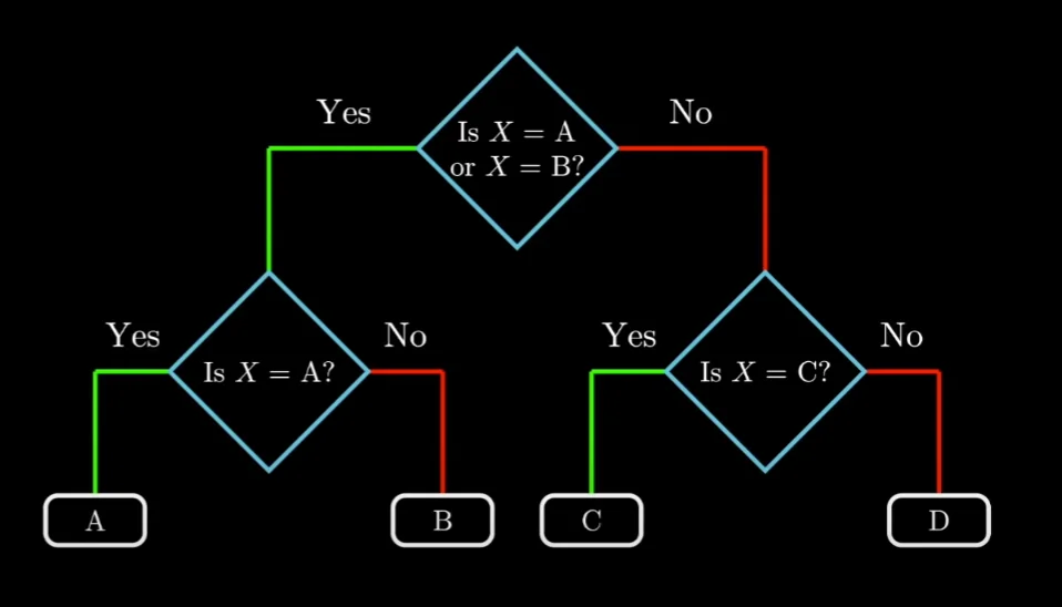
Representing the encoding as binary trees
In the above image, if we replace every left branch with 1 and every right branch with 0, we get a very interesting encoding. We get a prefix-free encoding that maps every character to a unique encoding. Given some bit string, all we have to do is start at the node and follow the bit string along the tree till we reach a leaf node. Every path to a leaf node in a tree is unique and hence our encoding is unique. Further, since it is on a tree and we stop only after reaching the leaf node, there can be no ambiguity. This means that the encoding is prefix-free!
In fact, for the above data, we can do no better than the encoding above. However, when we get to work with varying probabilities, things change. Shannon and Fano came up with an encoding that used the same concept of representing the encoding on binary trees to ensure they maintain the uniqueness and prefix-free requirements.
Their algorithm began by sorting the frequency of every event and then splitting the tree into two halves such that the prefix and suffix sum on either side of our division was as close to each other as possible. This had the intended effect of relegating lesser used symbols to the bottom (greater depth and hence longer encoding) and more frequently used symbols to shorter encodings. This was a big achievement and was known as the Shannon-Fano encoding for a long period of time. It was a good heuristic and performed well but it was not optimal.
Notice that with this greedy strategy, we cannot prove that it is taking the most optimal choice at the local level. This algorithm is not optimal.
At the same time, the Shannon-Fano encoding achieved both a unique representation of our data and more importantly, a prefix-free encoding that performed really well. Perhaps we can build upon their idea to obtain a prefix-free encoding with optimal compression.
Enter Huffman
Contrasting the top-down approach used by Shannon and Fano, Huffman viewed the problem with a slight change in perspective. Instead of trying to start at the root, he claimed that if we picked the least two probable events, then they must be at the bottom of the tree.
Locally optimal choice
We want lesser used symbols to have longer encodings. If the above was not true, then that would imply that there is a symbol with a higher frequency of occurrence that is now given a longer encoding. This increases the size of the compression and is hence not an optimal choice. We now know for a fact that the least used symbols must belong to the bottom of the tree.
Optimum Substructure
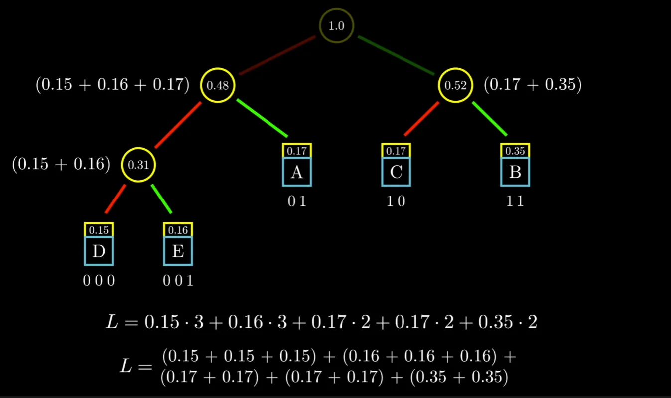
We can write $L = \sum_{i=1}^{n} p_i.d_i$ where $d_i$ is the depth of the $ith$ node in the tree. Note that this quantity $L$ is actually the same as the sum of the probabilities of every node except the root node in our tree. Consider the following example, notice that in the expanded view, the probability of each symbol gets included as many times as its depth in the tree.
Remember that our goal is to minimize L. Let our symbols have probabilities/frequency $p_1, p_2, \dots, p_k$ each and let us assume $p_1\leq p_2\leq\dots \leq p_k$. Using our optimal greedy choice, we can choose the bottommost nodes as $p_1+p_2$ and then restate the equation as follows.
$$ L(p_1,\dots,p_k) = p_1+p_2+L((p_1+p_2), p_3,\dots, p_k) $$That is, we have managed to express the next problem as a smaller version of the original problem for which we realize that again, the greedy choice holds. We have managed to obtain the optimum substructure in our problem.
This implies that therefore, our greedy algorithm is indeed correct. This is the Huffman encoding.
Given some text data in the form of $(data, frequency/probability)$ tuples we can build the Huffman tree by using the greedy logic described above. Always greedily pick the smallest two probabilities to form the leaf node, then repeat. This is guaranteed to give us the optimal solution.
It is interesting to note its similarity to Shannon-Fano encoding, sometimes, all you need is the slightest shift in perspective to solve some of the world’s unsolved problems :)
Huffman was able to prove that his encoding gives us the most optimal solution for encoding any set of $(data, probability)$ pairs as given. But… can we do even better? Theoretically no, but there are algorithms that can reduce the size of our data even more. The primary idea used by these algorithms is to chunk data into multiple byte chunks and then applying Huffman encoding. Note that while we mostly referred to ASCII text, Huffman encoding can be used to losslessly compress any form of binary data.
The following video was referenced while making this diary and is the source of some of the illustrations above, highly recommend watching this video.
References
These notes are old and I did not rigorously horde references back then. If some part of this content is your’s or you know where it’s from then do reach out to me and I’ll update it.
- Professor Kannan Srinathan’s course on Algorithm Analysis & Design in IIIT-H
- Huffman Codes: An Information Theory Perspective - Reducible