Amdahl's Law & Gustafson's Law
Interactive Graph
Table of Contents
Amdahl’s law
Before attempting to parallelize a program it’s a good idea to first measure the theoretical max speedup we can achieve by parallelizing our program. Further, note that the maximum speedup we can achieve depends on the amount of computing hardware available to run the parallel code. If I have 4 cores available I can only speed up the parallel code by 4 times. Amdahl’s law provides us with a function $S(n)$ which returns the theoretical speedup expected given expected $n$ speedup from computing resources.
Let our program consist of some code that executes serially and some code that executes in parallel. If we denote the serial part by $s$ and the parallel part by $p$, note that $s+p = 1 \implies s = 1 - p$.
Now, speedup $(S(n))$ is basically how much faster the program becomes, so if we consider the original execution time $T$ as $1$ unit of time then we can write the execution time on a parallel machine with $n$ cores as $T' = s + \frac{p}{n}$. Then the speedup,
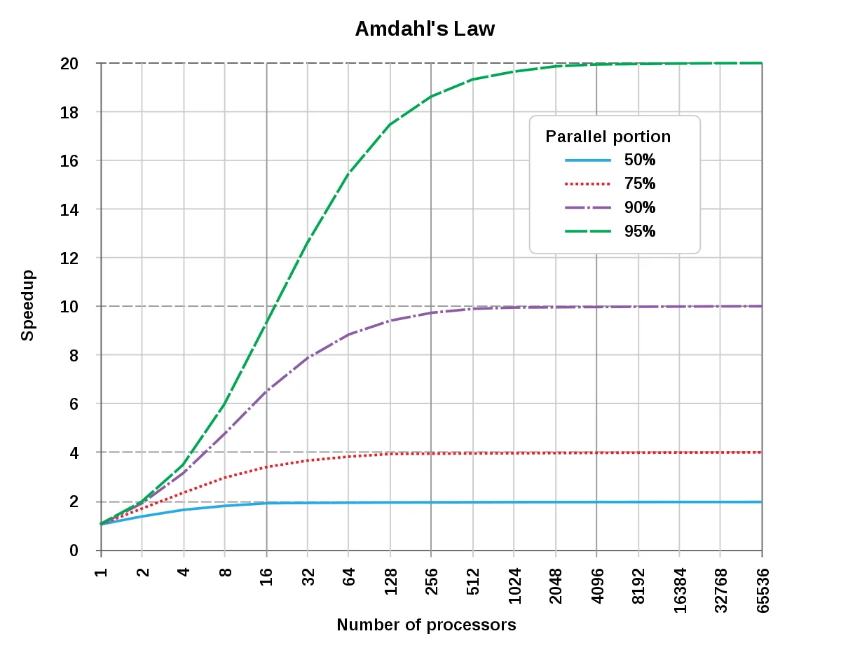
$$ S(n) = \frac{T}{T'} = \frac{s+p}{s + \frac{p}{n}} = \frac{1}{s + \frac{p}{n}} \\ \implies S(n) = \frac{1}{(1-p) + \frac{p}{n}} $$Note that the speedup $S(n)$ is bounded by $S(n) \leq \frac{1}{1-p}$.
Plotting Amdahl’s law for different values of $p$ gives us a graph that looks like this. Even with infinite computing power to instantly run all parallel code, our speedup will be bottlenecked by the serial portion of our program.
However, this fails to capture the general tendency most programmers have to increase problem size when given access to more computing power. This shortcoming was addressed by Gustafson’s law.
Gustafson’s Law
Gustafson’s law instead proposes that programmers tend to increase the size of problems to fully exploit the computing power that becomes available as the resources improve. Hence the speedup doesn’t necessarily “cap out” like predicted by Amdahl’s law. Programmers increase the problem size to benefit more from the increased parallel compute power.
If we increase the problem size, the portion of our program executing parallel code generally increases and hence benefits more. The speedup does not just cap out at some maximum if we do not assume a fixed problem size.
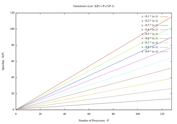
He proposed that $s+p=1$ be the fraction of time the program spends executing serial and parallel code respectively on a parallel machine. Then we have $T = s+np$. This gives us a speedup
$$ S(n) = \frac{T}{T'} = \frac{s+np}{s+p} = \frac{s+np}{1} \\ \implies S(n) = 1 + (n-1)p $$When the problem and system scale, the serial part (statistically) does not scale with them. Hence we get a linear relation between processor count and speedup. Quoting the Wiki,
The impact of Gustafson’s law was to shift research goals to select or reformulate problems so that solving a larger problem in the same amount of time would be possible. In a way, the law redefines efficiency, due to the possibility that limitations imposed by the sequential part of a program may be countered by increasing the total amount of computation.
We’ll discuss some cooler ways to extend these ideas in the case of task parallelism in Brent’s Theorem & Task Level Parallelism.
References
These notes are quite old, and I wasn’t rigorously collecting references back then. If any of the content used above belongs to you or someone you know, please let me know, and I’ll attribute it accordingly.