Preface

Before I get started… most of what follows is inspired by, and adapted from, notes I originally wrote back in high school (2019), now refreshed and digitized. These notes were first put together while following the now very famous Machine Learning specialization by Andrew Ng on Coursera, albeit a very old version. I would also highly recommend going over 3Blue1Brown’s lecture series on Neural Networks, they’re a delight to visual learners trying to understand back propagation better. I suppose I don’t really need to pitch Grant’s work much :’) but it’s genuinely amazing.

History

When learning a new topic, I always like to start with some history to understand the premise and “purpose” which lead to the creation of the given topic or field. In this case, “Artificial Intelligence” & “Machine Learning” have been fields of research since the 1950s.

The Turing Test

The world’s first computer was built in 1946, the ENIAC. But theoreticians like Turing had already been theorizing about (in his 1936 paper, On Computable Numbers, with an Application to the Entscheidungsproblem) a general purpose “universal machine” that could solve “computable” problems. It was also Turing who might have “kicked off” this field when he published his most cited paper, COMPUTING MACHINERY AND INTELLIGENCE in 1950, proposing the question “Can machines think?”

In this paper, he introduced the “Imitation Game” (now known as the Turing Test) as a practical way to assess if a machine could “think.” It remains a benchmark even today, while we continue to debate between “AI”, “AGI”, “ASI”, etc. His ideas drove a lot of curiosity into answering this question, “can machines think?”

The Dartmouth Conference

This is publicly recognized as the most well-known birthplace of AI. In 1956, John McCarthy, Marvin Minsky, Nathaniel Rochester, and Claude Shannon organized a large workshop to bring together leading researchers and formally established the field of AI as a dedicated area of study. This meeting marked the “official” birth of AI as a research field. John McCarthy is credited with coining the term “artificial intelligence.”

The Perceptron

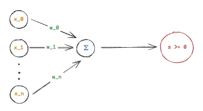
Following this conference, in 1957, Frank Rosenblatt built the world’s first perceptron. It was a (in today’s terms) single-layer neural network, which performed binary classification based on weighted inputs and a threshold. You can think of the first perceptron as something as simple as the following function:

Each input above ($x_i$) is assigned a weight ($w_i$). The perceptron calculates the weighted sum $\sum x_i \cdot w_i$. The red circle there is an “activation function.” For example, a simple binary classification function can be the following:

The perceptron can “learn” weights by adjusting its weights based on the “error” between its predicted output and the desired output. It was intended to be used in image recognition. This was a huge achievement at that time and sparked a lot of excitement about AI. However, people soon discovered that it could not learn more complex functions (for example, any non-linear function like the XOR), and no breakthroughs following the perceptron for many years to follow led to a period in tech known now as the “AI winter,” when interest and funding for AI research declined and very little progress was made.

From AI Winter to Deep Learning

Following this, several other breakthroughs were made in tech during the “AI winter.” Notably, the internet and the age of big data. Oh, also GPUs & Nvidia. Computing power increased at an exponential scale (Moore’s law), the world went online and huge amounts of data became widely available. This re-sparked the AI revolution. People were able to build much larger multi-layer perceptron networks and they were able to obtain the compute and data required to train them to compute much more complex functions now. We got Go & Chess engines better than any human in the world, and now we have the age of LLMs.

Linear Regression

Now that we know the history & motivation for “what” we’re trying to compute, let’s ground ourselves with a simple problem. One closely related to the perceptron’s early attempts at learning patterns.

Can we predict the relationship between a dependent variable ($y$, what we’re predicting) and one or more independent variables ($x_i$, the variables $y$ depends on), by fitting a linear equation to some observed data?

A Toy Problem

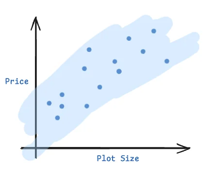
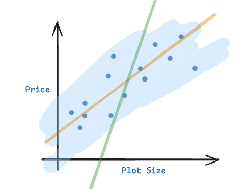
For example, let’s say we believe that housing prices are linearly dependent on the size of the plot. If we plot some data points of house sales, we may end up with a chart that looks as follows:

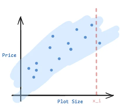
Looking at the above data, it’s reasonable to assume that housing prices are expected to linearly increase with increase in plot size. But if I wanted to know the best “expected” house price for a plot of size exactly $x_i$, how could I answer that question?

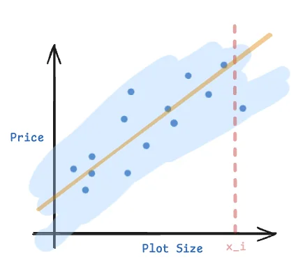
There’s no pre-existing data point with the exact value for plot size $x_i$, so I can’t regurgitate a known data point. Even if there was, it might be an outlier. I could find the best nearby $x_i$ and try to make a prediction, but what if I asked for a very large plot size? One which I did not have “nearby” pre-existing data points for? Like we mentioned previously, we could observe that the price $y$ appears to be linearly increasing with price $x$. We could then try to compute the “best-fit” linear equation to model this relationship. Let’s suppose we knew this “best-fit” line, given by some $f(x) = mx + c$.

We could then easily compute the best expected price for any given $x_i$. Awesome, but how do we compute this best fit line from our data? What does “best fit” even mean anyway?

Formalizing The Ideas

Let’s formalize some ideas from our discussion on solving the above problem. In the toy problem, we said that we were trying to predict housing prices as a function of plot size. In this case, housing prices are the value we want to predict.

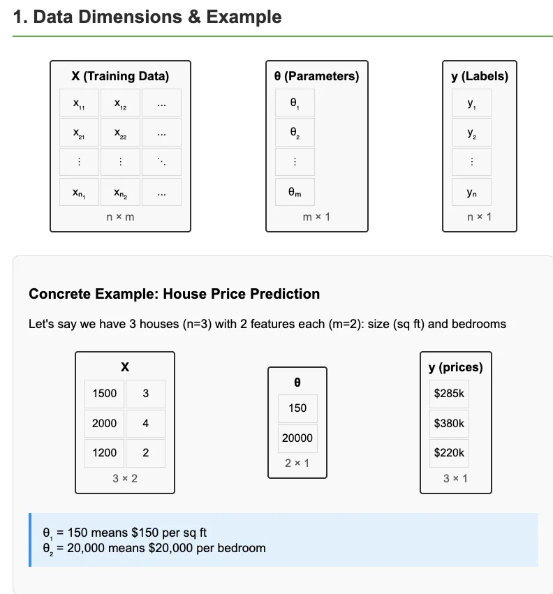
However, note that this value $y$ could be modeled to depend on $n$ different input variables. Think plot size, distance from the city, reputation of the builder, etc. Each of these input data points is called a feature. A feature is an individually measurable property or characteristic of the data that is used by the model to make predictions.

A single training example, $x^{(i)}$ is modeled as a vector of features. For example, $x^{(0)} = [1760 \text{ sqft.}, 11 \text{ km}, 4.6, \dots]$. Henceforth, we will use $x^{(i)}$ to refer to the $i^{th}$ training data point and $x_j$ to refer to the $j^{th}$ feature of training data point $x$. You can also use both notations together. So $x^{(i)}_j$ would refer to the $i^{th}$ training data point’s $j^{th}$ feature. $x$ itself will be a vector of features. $X$ will refer to the matrix of all $n$ training data points, where each row of $X$ is $x^{(i)}$.

The Hypothesis Function

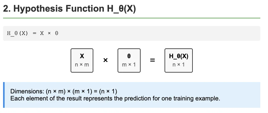
We can now define the hypothesis function $H_{\theta}(x)$ as the linear model we’re trying to learn. For a given input $x$ with $n$ features, our prediction is a linear combination of those features, weighted by our learned parameters $\theta$.

If we imagined $x$ and $\theta$ to both be 1-D vectors of size $n$, then the above equation is simply the dot product of both the vectors. So we can simplify the above equation to just:

In the above example, we have $n = 1$. So our hypothesis function $H_\theta(x)$ is simply $\theta_0 x_0 + \theta_1 x_1$. For simplicity, we make the convention to always set $x_0 = 1$. This gives us the simplified hypothesis function, $H_\theta(x) = \theta_0 + \theta_1 x_1$. In 2 dimensions, $\theta_0$ is simply the y-intercept and $\theta_1$ is the slope of the line.

The Cost Function

To learn the optimal parameters $\theta$, we need a way to measure how well our model is performing. Going back to the last question we raised when discussing the toy problem, “What does “best fit” even mean anyway?” In our toy problem, if we draw a couple of random lines onto the graph of data points,

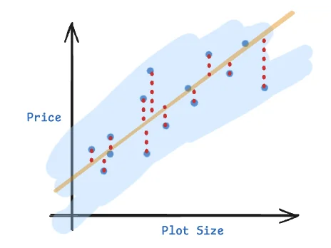
It’s easy to visually observe and claim that the orange line better “fits” the data than the green line. But how can we quantify this notion of “fit”? To solve this problem, we need to come up with a cost function. A cost function takes the training data points, and a predicted line of best fit as input, and outputs a quantifiable value for how “close” the line’s predicted values are to the actual training data points. Well one simple idea could be to simply compute the predicted value $y^{(i)}$ for each training data point $x^{(i)}$ using $H_\theta(x^{(i)})$ and compute the difference between the two values (well, the sum of the absolute values of the differences to be specific).

The cost function $J(\theta)$ would then be:

Note that we multiply the cost by $\frac{1}{n}$ here to normalize the error with respect to the number of available training data points. This function is called the Mean Absolute Error (MAE) and is a perfectly valid cost function. However, this function is mathematically / analytically a not-so-nice function to use to define the cost for linear regression. To “learn” the best fit parameters $\theta$, we usually use an algorithm that involves the computation of the differential of our cost function. The absolute value function $|x|$’s graph has a sharp corner at $x = 0$, which means its derivative is undefined at $x = 0$ and piecewise constant otherwise ($\pm 1$). This makes mathematically reasoning about it and gradient based optimization difficult. (It’s not possible to derive a simple closed-form solution for it, gradient based optimization might become unstable / harder to converge due to the sharp corner at $x = 0$.) Further, MAE would penalize all errors linearly. However, in most practical applications, we usually prefer penalizing “large” errors more “strongly.”

Due to these reasons, most popular implementations of linear regression implement a slightly different cost function called the Mean Squared Error (MSE). In principle, it’s very similar to MAE.

We simply swap the absolute value function $|x|$ for $x^2$. In contrast to MAE, this function’s differential is continuous and smooth. However, note that MSE will “punish” large errors more strongly than MAE. You’ll also notice that the denominator of our normalization fraction is now $2n$ instead of $n$. No significant reason for this. It’s just slightly more mathematically convenient to compute the derivative for this later.

We now have a simple, mathematical method to quantify how “good” or “bad” a set of learned parameters $\theta$ are for predicting some $y$ based on some training data $X$. That’s well and good, but we still need to solve the last part of this puzzle. How do we “learn” the best fit line, or the best set of parameters $\theta$ for minimizing the cost?

Gradient Descent

Finding the best set of parameters $\theta$ now just means finding the best values for $\theta$ that minimizes the value of the the cost function $J(\theta)$. So how do you find such a set of inputs $\theta$?

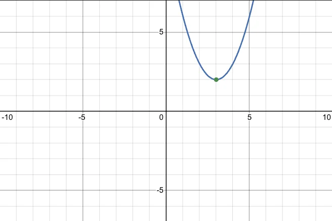
Consider the function $y = (x-3)^2 + 2$. We can find a minimum by differentiating it and setting $\frac{dy}{dx} = 0$. This gives us $\frac{dy}{dx} = \frac{d(x^2 - 6x + 9 + 2)}{dx} = 2x - 6 = 0 \implies x = 3$. At $x = 3$, $y = 2$. By double differentiating it, we get $\frac{d^2y}{dx^2} = 2 \gt 0$ which means it’s a minimum. Since this curve is concave-up shaped, it has just one minimum and hence it is the global minimum.

However, this same approach isn’t very feasible for more complicated functions. Sometimes solving for all possible values of $\frac{dy}{dx} = 0$ is difficult (or impossible). Checking the double derivative for complex functions might often be inconclusive and we may need to check higher order functions or use numerical methods. When we’re dealing with multiple variables and higher dimensional functions, the computations can get extremely complex and difficult to compute. So instead, people rely on iterative numerical optimization algorithms.

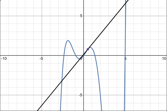
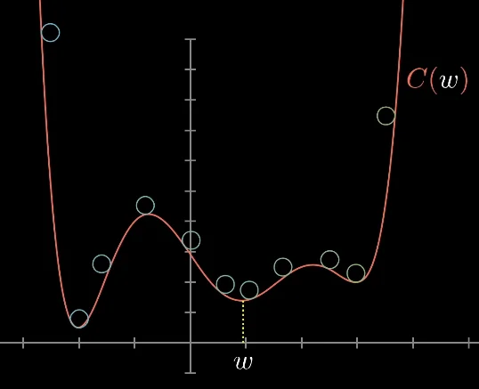
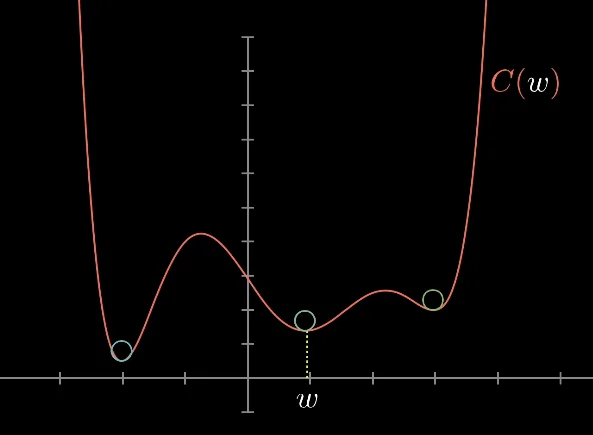
Gradient Descent is one such iterative optimization algorithm used to find the minimum of a function. We start with some random initial values for $\theta$ and repeatedly update them by taking small steps in the direction of the steepest descent of the cost function. Consider this more complex function below:

Given any point $w_0$, we can find out the answer to “Which direction should I move in to reduce the value of the function?” by computing the derivative (slope) of the function at that point $w_0$. If the slope is positive, we should move left to reduce the value of the function. If it’s negative, we should move right. If we do this repeatedly, we’ll eventually approach & reach some local minimum of the function. The visualization that really helps sell this idea is that of a ball rolling down the 2D hills (curves generated by the function). If we generate enough random initial points (or balls) and perform this procedure, we should eventually hit a very good local minimum.

• Pictures credit 3b1b: Gradient descent, how neural networks learn | Deep Learning Chapter 2

Gradient of A Function

This idea extends to $n$ dimensional spaces as well.

• Pictures credit 3b1b: Gradient descent, how neural networks learn | Deep Learning Chapter 2

Let’s formalize how we compute this gradient descent step for a multi-variate scalar function. Here are some terms to know:

1. Scalar Function: A function whose output is a single number, even if the input is multi-dimensional. For example: - $f(x) = x^2$ - $f(x, y) = x^2 - y^2$ - $f(x, y, z) = sin(x) + e^{y-z}$

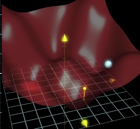
2. The Gradient of a Scalar Function: You can think of it as the $n$ dimensional (multi-variate) generalized case of the derivative of a 1D function. For a scalar function $f(x_1, \dots, x_n)$, the gradient is a vector representing the direction of steepest ascent of a function. Note that for 1D functions, the gradient was equivalent to the slope. However, even for a 2D function, notice that the “slope” or “gradient” must be a vector, since it has to point in a direction and have some magnitude associated with it. We compute the gradient of a multi-variate function as follows:

   $$ \nabla f(x_1, x_2, \dots, x_n) = \Big( \frac{\partial f}{\partial x_1}, \frac{\partial f}{\partial x_2}, \cdots, \frac{\partial f}{\partial x_N} \Big) $$

   In short, we take the partial derivative of $f$ with respect to each of the input dimensions. This final vector points to the direction of steepest ascent and its magnitude tells you the strength or steepness of that slope.

Note that we’ll cover the case of a non-scalar function later, when we cover Basics of Neural Networks.

The Algorithm

Going back to the original problem, we have our cost function:

And we’re trying to minimize it with gradient descent. The first step is to compute the gradient for this function, $\nabla_\theta J(\theta)$. If the number of parameters was only 1, then this would just be $\frac{dJ}{d\theta}$. Since $\theta$ is actually a vector of parameters, we need to compute it’s gradient, which is defined as the vector:

So what we need to compute here is the term $\frac{\partial J}{\partial \theta_i}$.

To compute the partial derivative here, we will use the chain rule. As a refresher, the chain rule states that if we have two functions $f$ and $g$ which are composed like $y = f(g(x))$, then the differential $\frac{dy}{dx} = \frac{dy}{dg} \cdot \frac{dg}{gx}$. In other words, the derivative is equal to the the derivative of the outer function evaluated at the inner function times the derivative of the inner function. Applying this here, we get:

To compute the last remaining partial derivative, notice that $y^{(i)}$ does not depend on $\theta_j$. Hence it’s derivative is $0$ with respect to $\theta_i$. Furthermore, if we expand $H_\theta(x^{(i)}) = \theta_0x^{(i)}_0 + \theta_1x^{(i)}_1 + \cdots + \theta_nx^{(i)}_n$, we can notice that most of these terms will go to 0. The partial derivative is therefore just $x^{(i)}_j$ ($\frac{d(cx)}{dx} = c$). With this, our final equation simplifies down to:

Now, all that remains is to define the “update” step that our algorithm will use to nudge the parameters $\theta$ in some direction based on the gradient of the cost function. We’ll define $\alpha$ to be the learning rate. It will be used to control the size of each step in our gradient descent. We can then define the update step as simply $\theta_j \coloneqq \theta_j - \alpha \cdot \frac{\partial J}{\partial \theta_j}$ which when expanded is:

By varying the size of $\alpha$, we can control how “large” the steps are that we take when attempting to find the local minima. With very small $\alpha$, we will make very incremental and slow progress towards the minima. With very large $\alpha$, we run the risk of missing the local optima altogether. But sometimes, larger $\alpha$ overshooting a local minimum might be useful to determine a better local minimum. In practice, we usually run several runs with different randomized initializations of $\theta$, and vary the step size from initially large values to smaller ones towards the end of the gradient descent process.

A Vectorized Implementation

Remember that $\theta$, $x^{(i)}$ and $y^{(i)}$ are all vectors. Computing each value by looping over each entry one by one is extremely slow. Each computation would occupy the use of 3 registers on the CPU, and we would likely need a lot of memory accesses. Instead, we have a lot of specialized hardware that is purpose built to compute operations such as these where we want to apply the exact same operation on a large amount of data. These operations fit nicely under SIMD from Flynn’s Taxonomy. In particular, we have a lot of purpose built libraries which are written to make maximum utilization of such specialized hardware for computing matrix-vector operations. Some more context on this in Mega-Project - kBLAS (Writing a Benchmark library in C & Optimizing L1, L2 Basic Linear Algebra Subprograms). I also intend to write a blog on GPUs soon. In short, we should try to write our operations as matrix-vector computations whenever possible. Let’s do this for linear regression.

First, let’s understand the dimensionality of our input & parameter vectors. Each of our training data points is a vector $x^{(i)}$ of dimensions $1 \times m$. We can encapsulate all of our training data inputs into a single matrix $X$ of dimensions $n \times m$. Here, each row of our matrix $X$ represents one of the training inputs. Each training input consists of $m$ features. For each training input $x^{(i)}$, we also have the training example’s correct output $y^{(i)}$ which is a vector of dimensions $n \times 1$. Note that whether it’s a row or column vector is just a choice that’ll help simplify the future expressions. Similarly we can represent our vector of hyper-parameters $\theta$ as a $m \times 1$ column vector (Thanks to Claude yet again for awesome visualizations…).

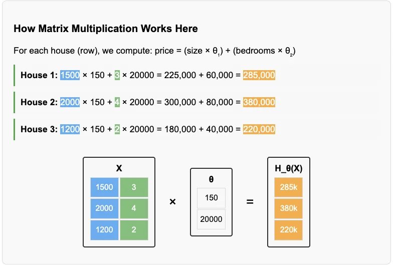
1. Our hypothesis function $H_\theta$ can be simply written as $H_\theta(x) = x \times \theta$. This would in essence, compute the $1 \times 1$ predicted output for a single input vector $x$. We can similarly model the computation for the entire training data matrix $X$ in one operation as well.

   

   

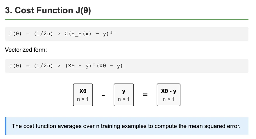
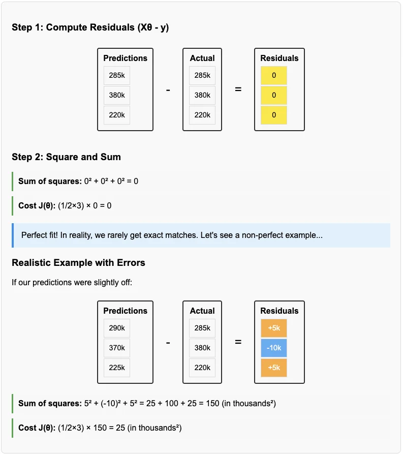
2. The cost function $J(\theta)$ can be written as $J(\theta) = \frac{\sum(H_\theta(x) - y)^2}{2n}$. $H_\theta(X)$ can be computed by multiplying the matrix $X$ with $\theta$ to give us the $n \times 1$ vector. After this, computing the numerator is a simple vector subtraction operation. We can then compute the square vector by computing $x^T \times x$. When $x$ is a row vector, it gives the sum of squares of the components of $x$. This is also known as the squared Euclidean norm of $x$.

   

   

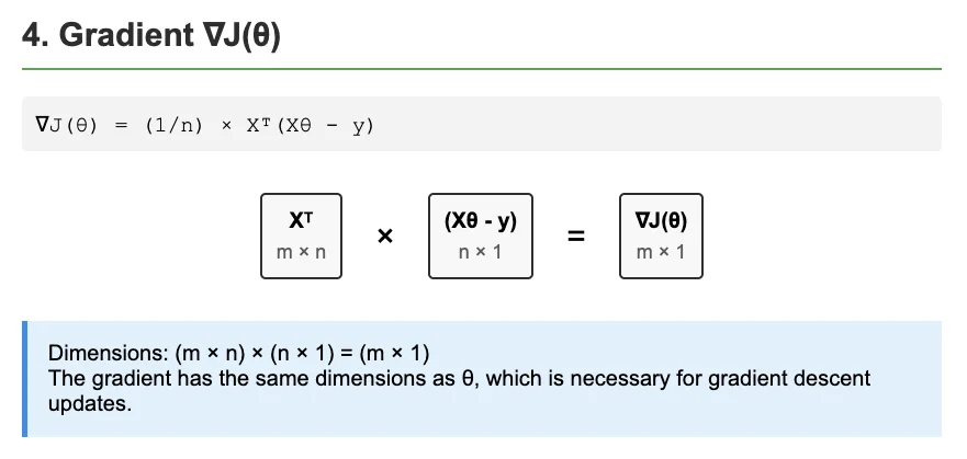
3. The gradient, $\nabla J(\theta)$ is then written as $\nabla J(\theta) = \frac{1}{n} \cdot (X^T \times (X \times \theta - y))$.

   

   

A PyTorch Implementation

I’m also attempting to learn PyTorch for the first time here, so I’ll be leaving some snippets here which I used to test and verify these implementations using PyTorch. To start off, let’s import the necessary libraries and set the seed for them to 42, just to make sure all experiments / findings from here are completely reproducible.

import torch
import torch.nn as nn # We'll need PyTorch for running the above algorithms
import numpy as np # Numpy for helping with plotting
import matplotlib.pyplot as plt # Matplotlib to actually plot graphs

torch.manual_seed(42)
np.random.seed(42)

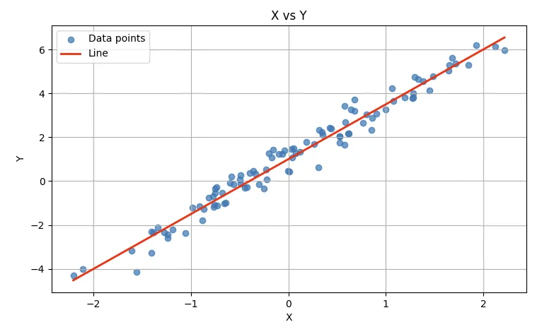
Next up, I’m going to create some sample training data by using a base function, say $y = 2.5x + 1$ and by adding some random noise to it. If you want to know what the function plot_xy does, I made a bunch of helper functions to quickly visualize plots. They’re mostly irrelevant.

# Let's make our sample data
NUM_SAMPLES = 100
NUM_FEATURES = 1
REAL_WEIGHT = 2.5
REAL_BIAS = 1.0

X = torch.randn(NUM_SAMPLES, NUM_FEATURES)
y = REAL_WEIGHT * X + REAL_BIAS + torch.randn(NUM_SAMPLES, 1) * 0.5 # The randn * 0.5 is our noise term

plot_xy(X, y, REAL_WEIGHT, REAL_BIAS)

The plot generated is as follows:

So far so good. We now need to create our model parameters, the model itself and pick the loss function and optimizer we want to use to learn our parameters. To do this in PyTorch we do the following:

# Initialize model, loss, and optimizer
model = nn.Linear(NUM_FEATURES, 1)
loss_function = nn.MSELoss()
optimizer = torch.optim.SGD(model.parameters(), lr=0.01)

Let’s train our model now for a 100 iterations of gradient descent.

# Let's train the model now
loss_log = []
NUM_EPOCHS = 100
for epoch in range(NUM_EPOCHS):
    # Forward pass
    y_pred = model(X)
    loss = loss_function(y_pred, y)

    # Backward pass
    optimizer.zero_grad()
    loss.backward()
    optimizer.step()

    # Log loss
    loss_log.append(loss.item())

learned_weight = model.weight.item()
learned_bias = model.bias.item()

print(f'\nReal parameters: weight={REAL_WEIGHT}, bias={REAL_BIAS}')
print(f'Learned parameters: weight={learned_weight:.4f}, bias={learned_bias:.4f}')
plot_loss(loss_log)

The output I get is:

Real parameters: weight=2.5, bias=1.0
Learned parameters: weight=2.2193, bias=1.0283

Not bad, but if I train for 1000 epochs instead of just 100, I’ll see a near perfect fit set of learned parameters instead:

Real parameters: weight=2.5, bias=1.0
Learned parameters: weight=2.5059, bias=1.0178

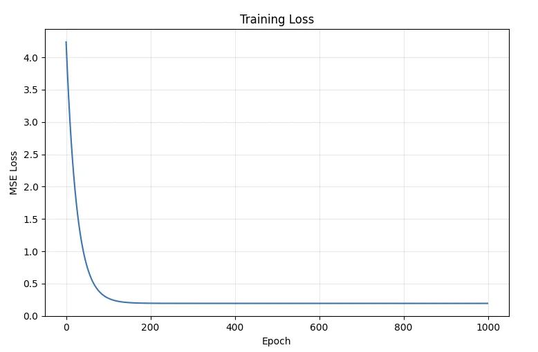
Plotting the loss (cost function) for our model over each epoch gives us the output we’d expect:

As we can see, a 100 epochs don’t seem to be enough to minimize the loss. We seem to have hit the minimum somewhere under the 200th epoch.

An Explanation Of The Code

I believe it’s also worthwhile to go over what some of these PyTorch functions do and how we’re using them to do linear regression. There’s a few things to note here:

1. torch.randn

   Returns a tensor filled with random numbers from a normal distribution with mean 0 and variance 1 (also called the standard normal distribution). That is, $\text{out}_i \sim \mathcal{N}(0, 1)$

   In short, when we write torch.randn(a, b), we’re creating a tensor of size $a \times b$ where each element of this tensor is sampled from the standard normal distribution with mean $0$ and variance $1$.

2. torch.nn.Linear

   Applies an affine linear transformation to the incoming data: $y=xA^T+b$

   Linear accepts the dimensions of the input feature vector and the output feature vector. In our case, our input features (say plot size) was just 1 and the size of the output feature (say house price) was also 1. By default, the argument bias=True is set. This means the Linear class automatically maintains a bias term in the network (technically Linear is actually implementing Neural Network (see: Basics of Neural Networks) which implements an affine transform), but for our use case, they’re equivalent. The bias term is our + c term. This is useful because it lets the model better fit data that is not normalized around the origin. The matrix $A$ is the parameter matrix (a vector for 1D output features).

   The model stores the parameters internally and makes them accessible via model.weight and model.bias. These are torch.Parameter objects, which are special tensors that PyTorch knows to track for gradient calculations.

3. nn.MSELoss

   Creates a criterion that measures the mean squared error (squared L2 norm) between each element in the input $x$ and target $y$.

   This just defines / implements the same MSE error function we defined earlier. Note that PyTorch likely does not use the $\frac{1}{2n}$ term to normalize and uses $\frac{1}{n}$ instead. You can also pass in reduction='sum' to have the cost function skip division (which can be unstable / slow) and just compute the sum of the MSE terms instead. However, with sum, note that increasing training data / batch size implies an increase in loss / gradient size and would likely need tuning of the learning rate $\alpha$ dependent on the batch size to work well.

4. torch.optim.SGD

   Implements stochastic gradient descent (optionally with momentum).

   There’s not much to explain here. Given that we’ve defaulted weight_decay and all the other fancy modifiers to $0$, it’s implementing exactly the same gradient descent algorithm we’ve described above.

   However, there are some important implementation details to note. model.parameters() returns an iterator over all learnable parameters in the model. The optimizer stores references to these parameters and will update them in-place during optimizer.step(). One more thing, you may have noticed that we have a line optimizer.zero_grad() before we perform the step(). This is because PyTorch accumulates gradients by default. There’s some reasons for this, which I hope to go over in Basics of Neural Networks.

5. The computation graph: There’s one part of the above snippets that might look weird / unrelated to new learners.

    # Forward pass
    y_pred = model(X)
    loss = loss_function(y_pred, y)
   
    # Backward pass
    optimizer.zero_grad()
    loss.backward()
    optimizer.step()
   

   loss appears to be computed independently and seems to be a simple output tensor. We then call loss.backward()… which should do nothing? And then we call optimizer.step()? Will it still work if I just remove the loss.backward() line? How does loss even inject itself into the code flow / path of the optimizer?

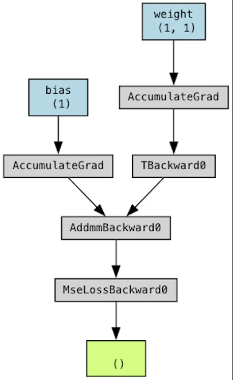
   Turns out, every tensor in PyTorch can track how it was created. y_pred.grad_fn would contain a reference to the objects it was computed from. PyTorch essentially maintains a dynamic computation graph built on-the-fly as you do operations. We can actually visualize this graph using torchviz. Let’s execute this piece of code:

   from torchviz import make_dot
   import torch
   import torch.nn as nn
   
   model = nn.Linear(1, 1)
   X = torch.tensor([2.0](/blog/2-0))
   y = torch.tensor([5.0](/blog/5-0))
   
   y_pred = model(X)
   loss = nn.MSELoss()(y_pred, y)
   
   # Create visualization
   dot = make_dot(loss, params=dict(model.named_parameters()))
   dot.render("graph", format="png")  # creates graph.png
   

   We get the following graph.png:

   

   So when you call loss.backward(), it actually goes backward through this graph and computes the gradient of y_pred with respect to weight and bias and stores these gradients in the .grad attribute of each parameter. These are then picked up by the optimizer when we run optimizer.step(). There’s more details to this, but maybe in a future blog :)

Some More Experiments

As we saw above, tweaking the number of epochs we trained for gave us significantly better results than without. You’ll notice there are some more arbitrary constants sprinkled into the code. What about the value of the learning rate? How do these values all affect our final set of learned parameters $\theta$? To answer this, we can run a few experiments. Let’s first modularize our training code:

# Let's train the model now
def train_and_log_params(lr=0.01, num_epochs=100):
    # Reinitialize model / optimizer & create log stores
    model = nn.Linear(NUM_FEATURES, 1)  
    optimizer = torch.optim.SGD(model.parameters(), lr=lr)
    loss_function = nn.MSELoss()
    loss_log, weights_log, biases_log = [], [], []

    for epoch in range(num_epochs):
        # Forward pass
        y_pred = model(X)
        loss = loss_function(y_pred, y)

        # Log values
        loss_log.append(loss.item())
        weights_log.append(model.weight.item())
        biases_log.append(model.bias.item())

        # Backward pass
        optimizer.zero_grad()
        loss.backward()
        optimizer.step()

    return loss_log, weights_log, biases_log

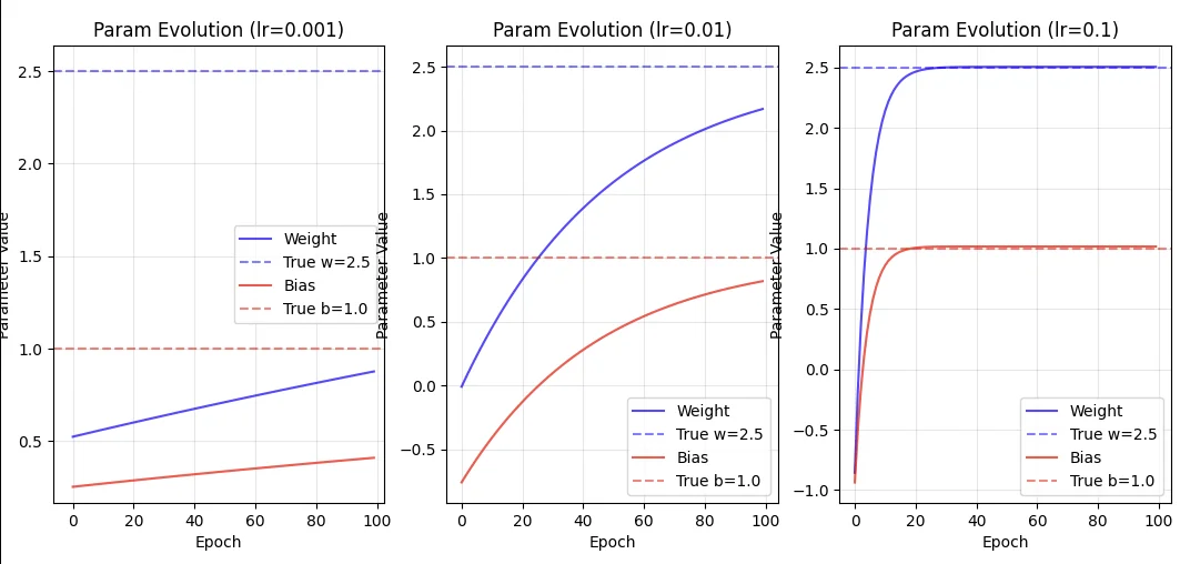
Now, we can vary a bunch of stuff and see how loss and our parameters vary with them. For example, let’s try varying the learning rate $\alpha$.

# Let's try varying learning rates
learning_rates = [0.001, 0.01, 0.1]
data = {}
for lr in learning_rates:
    _, weights_log, biases_log = train_and_log_params(lr)
    data[lr] = (weights_log, biases_log)

plot_param_evolution(data, REAL_WEIGHT, REAL_BIAS)

Here’s what we get. For very small learning rate and just 100 epochs, both $\alpha = 0.001$ and $\alpha = 0.01$, the weights and bias fail to converge to the “real” values. We need the much higher rate $0.1$ to converge quickly.

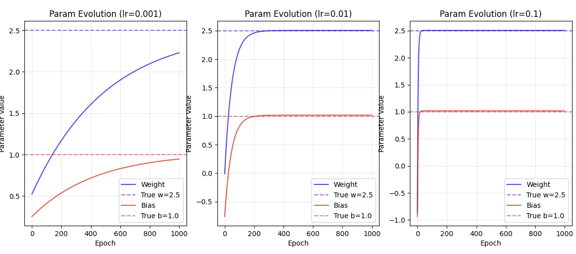
If we increased the number of epochs to 1000 however,

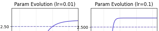
You’ll notice that $\alpha = 0.01$ is sufficient, but $\alpha = 0.001$ still fails to converge! Looking at the evolution further, you’ll notice that

The larger learning rate has chosen a slightly worse optimum, but it did reach there a lot faster than $\alpha = 0.01$. That’s the tradeoff we make here.

And that’s about it for linear regression. Next up, in Basics of Supervised Learning - Logistic Regression, we’ll be expanding the ideas we learnt in this blog to train logical classifiers, where we’ll see how a simple modification to our linear model - adding a non-linear activation function - transforms our regression problem into a powerful classification tool that will help us bridge the gap between linear models and the neural networks that eventually conquered the limitations of Rosenblatt’s perceptron.