Preface & References

I document topics I’ve discovered and my exploration of these topics while following the course, Algorithms for DNA Sequencing, by John Hopkins University on Coursera. The course is taken by two instructors Ben Langmead and Jacob Pritt.

We will study the fundamental ideas, techniques, and data structures needed to analyze DNA sequencing data. In order to put these and related concepts into practice, we will combine what we learn with our programming expertise. Real genome sequences and real sequencing data will be used in our study. We will use Boyer-Moore to enhance naïve precise matching. We then learn indexing, preprocessing, grouping and ordering in indexing, K-mers, k-mer indices and to solve the approximate matching problem. Finally, we will discuss solving the alignment problem and explore interesting topics such as De Brujin Graphs, Eulerian walks and the Shortest common super-string problem.

Along the way, I document content I’ve read about while exploring related topics such as suffix string structures and relations to my research work on the STAR aligner.

Algorithms for Exact Matching

The Naive Algorithm

The naive algorithm is trivial and simply scans the main text $S$ for the pattern $T$ in a quadratic manner by just iterating over each character of the main text for the starting position and comparing it with the pattern text $T$ character by character. This is clearly extremely inefficient and has a worst case running time complexity of $O(nm)$. A simple example where such a run-time is possible is the strings.

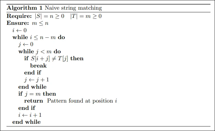
Boyer-Moore Pattern Matching

Boyer Moore algorithm starts matching from the last character of the pattern. It uses two main heuristics to solve the problem.

• Bad Character Rule: If we do some character comparisons, and we find a mismatch, we will skip all alignment checks until one of two things happens. Either the mismatch becomes a match, or the pattern $T$ moves all the way past the mismatched text character.

  

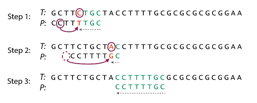
  Explanation: Our mismatching character is "C". We then search $T$ for the last occurrence of "C". Then we will shift $T$ by $3$ such that "C" is aligned between $S$ and $T$

• Good Suffix Rule: Let $t$ represent the longest common suffix matched by our pattern $T$ with the portion of $S$ we are checking for a match with. We can now skip all comparisons until either there are no mismatches between $S$ and $t$ or $S$ moves past $t$. This can be done relatively fast with some pre-processing.

  

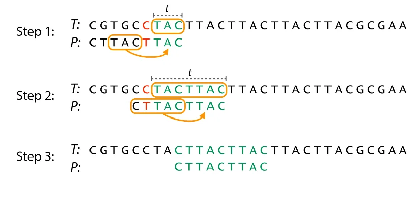
  Explanation: We have a sub-string $t$ of $T$ matched with pattern $S$ (in green) before a mismatch. We then find an occurrence of $t$ in $S$. After finding this, we jump checks to align $t$ in $S$ with $t$ in $T$.

The algorithm simply tries both heuristics and picks the maximum skip distance returned by both.

Booyer-Moore Performance:

• Worst-case performance: $\Theta(m)$ pre-processing $+ O(mn)$ matching.

• Best-case performance: $\Theta(m)$ pre-processing $+ \Omega(\frac{n}{m})$ matching.

• Worst-case space complexity: $\Theta(k)$

The traditional Boyer-Moore technique has the drawback of not performing as well on short alphabets like DNA. Because sub-strings recur often, the skip distance tends to cease increasing as the pattern length increases. One can however acquire longer skips over the text at the cost of remembering more of what has already been matched.

Knuth-Morris-Pratt Pattern Matching (KMP)

KMP is a string matching algorithm that reduces the worst case time complexity of the pattern finding problem in a given text to $O(n+m)$. The idea behind KMP is pretty simple. We discuss it in the following sections.

Prefix Function

Given a string $s$ such that $|s| = n$, we define the prefix function of $s$ as a function $\pi$ where $\pi(i)$ is the length of the longest proper prefix of the prefix sub-string $s[0:i]$. Here $s[0:i]$ refers to the sub-string starting at (zero-indexed) index $0$ and ending at index $i$, both inclusive. A prefix that is distinct from the string itself is a proper prefix. We define $\pi(0) = 0$. We usually compute the prefix function as an array $\pi$ where $\pi[i]$ stores the value of $\pi(i)$.

More formally, we define the prefix function as:

For example, prefix function of string “abcabcd” is  $[0, 0, 0, 1, 2, 3, 0]$ , and prefix function of string “aabaaab” is  $[0, 1, 0, 1, 2, 2, 3]$ .

The naive way to compute this array is to simply iterate on each prefix starting position, the prefix length and then compare sub-strings. This gives us a worst case time complexity of $O(n^3)$ which is clearly pretty poor.

Optimizations

• Prefix function values can only increase by a maximum of one between consequent indices.

  Proof by contradiction: If $\pi[i + 1] \gt \pi[i] + 1$, we may take the suffix ending in position $i + 1$ with the length $\pi[i + 1]$ and delete the final character from it. We then get a suffix that ends in position $i$ and has the length $\pi[i + 1] - 1$, which is preferable to $\pi[i]$.

  The prefix function’s value can therefore either increase by one, remain unchanged, or drop by a certain amount when going to the next slot. The function can only increase by a total of $n$ steps and can only decrease by a total of $n$ steps. This means that we only really need to perform $O(n)$ string comparisons. This reduces our time complexity to $O(n^2)$.

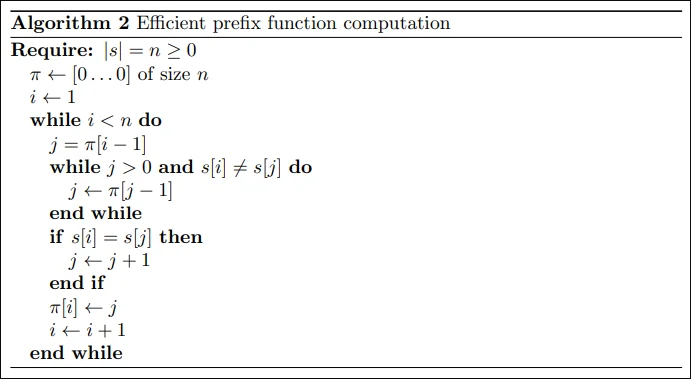
• We use dynamic programming to store the information computed in previous steps. Let’s say we have computed all values of $\pi$ till $i$ and now want to compute $\pi[i+i]$. Now we know that the suffix at position $i$ of length $\pi[i]$ is the same as the prefix of length $\pi[i]$. We get two cases:

  1. If $s[i+1] = s[\pi[i]]$ , this implies that $\pi[i+1] = \pi[i] + 1$.

  2. If  $s[i+1] \neq s[\pi[i]]$ , we know we have to compare shorter strings. We want to move quickly to the longest length $j \lt \pi[i]$ , such that the prefix property at position $i$  holds ( $s[0 \dots j-1] = s[i-j+1 \dots i]$ ). This value ends up being  $\pi[j-1]$ , which was already calculated.

The final algorithm looks something like this:

Efficient Pattern Matching

To do this task fast, we simply apply the prefix function we discussed above. Given the pattern $t$ and main text $s$, we generate the new string $t + \# + s$ and compute the prefix function for this string.

By definition  $\pi[i]$ is the largest length of a sub-string that coincides to the prefix and ends in position $i$. Here this is just the largest block that coincides with  $s$  and ends at position  $i$ , this is a direct implication of our separation character $\#$. Now, if for some index $i$, $\pi[i] = n$  is true, it implies that  $t$  appears completely at this position, i.e. it ends at position  $i$ .

If at some position  $i$  we have $\pi[i] = n$ , then at position $i - (n+1) - n + 1 = i - 2n$ in the string  $s$  the string  $t$  appears. Therefore we just need to compute the prefix function for our generated string in linear time using the above mentioned algorithm to solve the string matching problem in linear time.

Time complexity: $O(|s|+|t|)$

Comparison of Both

Source: What are the main differences between the Knuth-Morris-Pratt and Boyer-Moore search algorithms? - StackOverflow

• Boyer-Moore’s approach is to try to match the last character of the pattern instead of the first one with the assumption that if there’s not match at the end no need to try to match at the beginning. This allows for "big jumps" therefore BM works better when the pattern and the text you are searching resemble "natural text" (i.e. English) Boyer-Moore example run through

• Knuth-Morris-Pratt searches for occurrences of a "word" W within a main "text string" S by employing the observation that when a mismatch occurs, the word itself embodies sufficient information to determine where the next match could begin, thus bypassing re-examination of previously matched characters. KMP example run through

This means KMP is better suited for small sets like DNA (ACTG)

Offline Algorithms: Indexing and k-mers

A few more ideas we can use when working with pattern matching problems is grouping and indexing. In essence, we can enumerate all sub-strings of some constant length (say 5) from the main text and store this in an vector for example. We call these sub-strings of some constant length $k$ a \textbf{k-mer}. The stored index of the k-mer contains the indices at which it is found in the main string.

Now as for how we quickly search for a k-mer in this pre-processes data, we have two options.

• Binary search. We store the pre-processed data in sorted order. Can be done online during the pre-process stage or later be sorted after collection. Once done, finding a query k-mer simply involved binary searching on this sorted array. Note that strings can always be sorted by lexicographic order, this means that they will form a monotonous sequence for our query k-mer which means that our binary search is guaranteed to succeed in $O(log(n))$ comparisons. Each comparison can at worst case be $O(k)$. Hence we have a total time complexity of $O(klog(n))$. Here $n$ is the number of k-mer’s we have pre-processed.

• Hashing. Here, we hash each k-mer using some well known hashing function such as djb2, murmur, Fibonacci hashing, etc. to quickly query their existence into a hash-table. Various types of hash-tables can be used, Cuckoo, Robin-Hood, etc. This is pretty much just using the already existing plethora of literature on the subject of hashing to help speed up the algorithm. Worst case time complexity is $O(k*c)$ where $c$ is the constant involved with hashing. Note that this constant can have varying degrees of performance based on factors such as the number of k-mers stored, etc.

• Tries. Another data structure that I believe would be useful here is a Trie. Tries are a type of tree data structure that are used for efficient data insertion, searching, and deletion. Tries are also known as prefix trees, because they store data in a way that allows for fast search operations based on prefixes of keys. A k-mer trie is a specific type of trie data structure that is used to store and search for k-mers, which are sub-strings of a fixed length $k$ in a given string. The k-mer trie data structure allows for efficient searching of k-mers within a string, and can be used in applications such as sequence alignment and gene prediction. Time complexity is $O(k)$ for each query operation.

Further k-mer optimizations

Notice that one of the main bottlenecks here is the number of k-mers we have to store in our pre-processed data structure. Since the k-mers have a lot of overlap, one idea might be to reduce the number of k-mers we have to store in half by storing only those k-mers which start at odd indices. A consequence of this however, is that now our match success rate is only $50\%$. However, we can get back to a $100\%$ success rate by realizing that all we have to do is query indices which cover the entire field $\mod \ 2$ around the query index $q_i$.

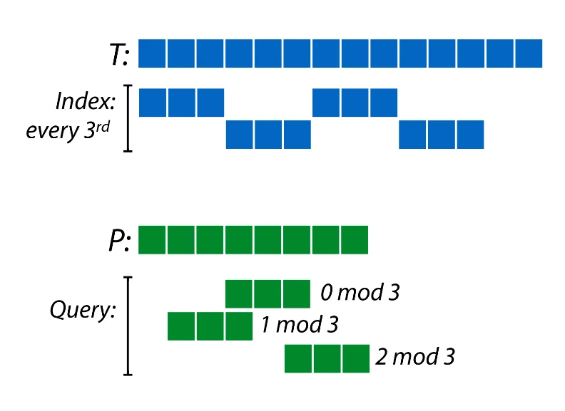
For example, if we store only $\frac{1}{3}^{rd}$ the number of k-mers, one way to do it would be to store every kmer which starts at a position $0 \ \mod \ 3$. Now we just query indices around $q_i$ which give us the entire field $Z_3$ when taking indices $\mod \ 3$. Now we just check for existence of prefixes and suffixes as required for the required types of kmers and verify existence of the actual query string.

Here we are paying extra penalty during the query phase for reducing the pre-process time. Further, pre-processing larger number of kmers usually requires more memory and this consequently leads to major penalty during the query phase due to terrible caching of the pre-processed data. So often it is worth the extra penalty paid during query operations to reduce the size of the pre-processed data simply to benefit from cache optimizations.