Brent's Theorem & Task Level Parallelism
Interactive Graph
Table of Contents
Suggestion for digging deeper into HPC ideas: https://ocw.mit.edu/courses/6-172-performance-engineering-of-software-systems-fall-2018/pages/syllabus/
Modeling task-level parallelism as a DAG (Directed Acyclic Graph)
One major issue we had with the OMP parallel execution model was the use of an implicit barrier at the end of every parallel block. Essentially, there is a period of time where the CPU spends time waiting for all the parallelly executing threads to join. This gives us moments of time where we are sitting idling and wasting precious compute time. One idea to solve this problem is to allow threads to keep executing without waiting for a join. Note that a thread $A$ only needs to wait on a thread $B$ when $B$ is still computing some data that $A$ needs to continue execution.
Hence $A$ can keep executing until it hits such a dependence barrier. Following this idea, we can always construct a dependency DAG of all the parallel workloads in a problem.
It allows us to come up with the following theoretical formulation of parallelization and speedup.
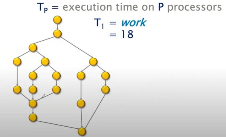
Let’s say each node in the graph represented one unit of work. In the above graph, I have $18$ units of work. If I executed the entire program serially, $T_1 = W = 18$. Assuming 1 unit work per 1 unit time, $T_1$ which is the serial execution time is $18$. To compute speedup, I want to be able to compute $\frac{T_1}{T_p}$, where $T_p$ is the execution time on $p$ processors.
Here, we establish 2 lower bounds on the value of $T_p$. First, assuming uniform compute power across all processors, $T_p \geq \frac{T_1}{p}$. If each core took up an equal portion of the work it would need at least this much time to compute.
Next, we introduce the idea of the critical path in the graph. The critical path is the length of the longest dependency chain in the graph. Note that no matter what, dependencies must be processed in a topological ordering and we cannot skip serially executing this portion of our code. This allows us to establish another lower bound $T_p \geq T_\infty$.
Here $T_\infty$ is the span or critical path length of the graph. Essentially the minimum time required if we had access to infinite parallel processing which eliminated the cost of processing everything except the critical path.
We call these the Work law and the Span law.
$$ T_p \geq \frac{T_1}{p} \\ T_p \geq T_\infty \\ T_p \geq max(\frac{T_1}{p}, T_\infty) $$Now, we compute speedup as just $S = \frac{T_1}{T_p}$. The maximum speedup is the case where we have infinite parallel computing power and here we are only limited by the span law. Hence maximum possible speedup is
$$ S_{max} = \frac{T_1}{T_\infty} $$Introducing some notation, we will now refer to the work required to be done as $W(n)$ and the span of the dependency DAG of this work as $D(n)$. The time for completion is $T(n)$. We now introduce the concept of average parallelism. Intuitively we can think of this as the amount of parallel work we can get done per critical path vertex.
$$ Avg. \ Parallelism = \frac{W(n)}{D(n)} $$It is possible to prove that there always exists an alignment of nodes in a DAG such that we can essentially partition the DAG into levels separated by the nodes on the critical path in the DAG.
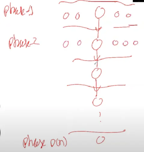
This is what we’d like to define as “average parallelism.”
If we define $W_i$ as the work done in ‘each phase’ then it follows that $W(n) = \sum_i^{D(n)} W_i$ and $T(n) = \sum_i^{D(n)} \lceil \frac{W_i}{p} \rceil$.
Brent’s Theorem
These two formulations essentially give us Brent’s theorem
$$ W(n) = \sum_i^{D(n)} W_i \\ T(n) = \sum_i^{D(n)} \lceil \frac{W_i}{p} \rceil \\ \implies T(n) \leq \sum_i^{D(n)} (\frac{W_i - 1}{p} + 1) = \frac{W(n) - D(n)}{p} + D(n) \\ \implies T(n) \leq \frac{W(n)}{p} + \frac{D(n)(p-1)}{p} \\ \implies T(n) \leq \frac{W(n)}{p} + \approx D(n) $$For the last step, we approximate the fraction to be $1$. This is the upper bound given to us on $T(n)$ by Brent’s law. Combining both laws, we get
$$ max(\frac{T_1}{p}, T_\infty) = max(\frac{W(n)}{p}, D(n) \leq T(n) \leq \frac{W(n)}{p} + D(n) $$This tells us that $T(n)$ must be within a factor of two from $\frac{W(n)}{p}$.
We can also write Brent’s theorem as
$$ T(n) \leq \frac{T_1(n)}{p} + T_\infty $$If our sped-up time $T(n)$ is greater than this upper bound then it implies that we are not doing a great job at parallelizing our workload. Whereas, if it is within the given bounds then we can say that the work is provably optimal.
Speedup and Work Optimality
When measuring speed up, it becomes very important that we take into consideration the best time of execution by a serial algorithm and compare it against parallel performance.
Essentially, we will write speedup as $S = \frac{T_*(n)}{T_p(n)} = \frac{W_*(n)}{T_p(n)}$ where the subscript * means best score by a serial algorithm for the same task.
This lets us get the following derivation,
$$ \begin{aligned} S_p(n) = \frac{W_*(n)}{T_p(n)} \\ \implies S(n) \geq \frac{W_*(n)}{\frac{W_p(n)}{p} + D_p(n)} = \frac{W_* \times p}{W_p + D_p \cdot p} \\ \implies S(n) \geq \frac{p}{\frac{W_p}{W_*} + \frac{D_p \cdot p}{W_*}} \end{aligned} $$For ideal speedup, we want the denominator to be as close to 1 as possible. This means $W_p \approx W_*$ is very good for us. Further, $\frac{W_*}{p}$ must steadily grow with $D_p$.
The first implication is fairly intuitive, we shouldn’t have to do extra work as we parallelize more. That is, parallel work $W_p$ shouldn’t scale with $W_*$ otherwise we’ll have to keep doing more work as we increase parallelization.
The second implication intuitively means that the ‘work per processor’ should grow proportional to span. That is, we shouldn’t be in a situation where $D_p$ (the span) increases but work per processor doesn’t, otherwise a lot of parallel compute power is wasted over waiting for the span to finish execution.