Previously, we discussed a dynamic programming solution to solve Levenshtein Edit Distance. Today, we’ll look at another interesting problem.

Chain Matrix Multiplication / Parenthesization

The problem

The problem of chain matrix multiplication is quite interesting. We previously saw that the best-known algorithms for multiplying two matrices are around the order $O(n^{2.81})$, This is not very ideal, especially for multiplying a chain of matrices. However, there is something we can do to severely save computing power!

Consider the following problem.

Because the multiplication is associative, we can choose what multiplication we wish to perform. That means, we can do both of the following.

$(A \times B) \times C$ and $A \times (B\times C)$. Notice that if we did the former, our first computation would give us a $20 \times 20$ matrix which must be multiplied with a $20 \times 1$ matrix. This will give Strassen’s input of the order $O(n^2)$.

However, if we picked the alternate route, after the first multiplication, we would have a $1\times1$ matrix to be multiplied with a $20 \times 1$ matrix. This is far more superior and will help reduce the input sizes of the matrices we perform multiplication on as this gives Strassen’s input only of the order $O(n)$.

This is the core idea of chain matrix multiplication. A more general term for this problem can be “Parenthesization.” It simply asks the question, “For some associative computation where each computation takes some cost $c$ to compute, what is the minimum cost I can incur in total for my total computation by just reordering the computation by rules of associativity?”

How do we approach this?

We realize pretty quickly that greedy approaches will not work here. There is no notion of the locally optimal solution. Even if we pick the first pairing to be the one that gives the least cost it says nothing about how this pick affects the later picks. Hence we must try them all out.

What about DP?

How can we effectively exploit some substructure of this problem to write a recursive solution?

Let’s say we’re given a sequence of $n$ matrices to multiply $a_0 \times a_1 \times \dots \times a_{n-1}$.

Notice that at any given point, we can use the following idea to divide the problem into sub-problems. For any given continuous sub-segment, I must divide it into a multiplication of exactly two segments. For the above sequence, let the optimal pairing be $[a_0 \dots a_i]\times[a_{i+1} \dots a_{n-1}]$. Then this is the split that I must perform at this state.

How do I know what the optimal split is? I must simply try all possible positions for the split all the way from between $a_0$ , $a_1$ to $a_{n-2}$ , $a_{n-1}$. To “try” each of these possible positions, I must know beforehand the cost of calculating each subpart.

So far we’ve seen examples of prefix and suffix dp. In the LIS problem, we calculated the LIS for every prefix. For edit distance, we could’ve done it either using a prefix or suffix dp. However, we quickly realize that this problem does not have that kind of structure. It is a lot more difficult to draw the DAG structure for this problem as this problem does not have a very “linear” way of solving it. Notice that our solution essentially requires us to compute the minimum cost for each and every “sub-segment” in our array of matrices.

Arriving at the DP solution

Let’s try to answer the following questions as we try to arrive at our DP solution.

1. What is the number of subproblems?

   As stated previously, we need to compute the optimal cost of multiplying every “subarray” of matrices. For some given array of length $N$ we can have $\frac{N \times (N+1)}{2}$ such sub-segments. (We will have 1 segment of length $N$, 2 of length $N-1$, etc. Which gives us a total of $\sum_{i=1}^{n}i$)

   Hence our sub-problems are of the order of $O(n^2)$. Our DP will likely be at least of $n^2$ complexity.

2. Find the solution at some state and count the number of possibilities we have to brute force over

   At some given state, notice that we are trying to compute the minimum cost required to multiply an ordered list of matrices from $[a_i\dots a_j]$. To do so, we must brute force over all possible splits of this sub-array. The following pseudo-code will paint a better picture.

   for k in [i, j-1]:
   		DP[i][j] = min(DP[i][j], DP[i][k] + DP[k+1][j] + cost(M[i][k], M[k+1][j])
   

   Here, $DP[i][j]$ stores the minimum cost incurred in optimally multiplying the segment from $i \to j$ and cost simply calculates the cost of multiplying the resultant two matrices $[a_i \dots a_k]\times[a_{k+1}\dots a_j]$.

   Notice that for any given $i, j$ there are a linear number of problems we must brute force over. Hence this step of our algorithm will have $O(n)$ time complexity.

3. Finding the recurrence

   We already derived the recurrence to explain the previous point better. The recurrence is the same as the one given in the pseudo-code. Each of the $DP[i][k]$ and $DP[k+1][j]$ states there represents the solution to one of its sub-problems.

4. Figuring out the DAG structure and making sure we don’t have any cycles

   This turns to be a lot messier and harder to work with for substring/subarray dp as compared to prefix/suffix dp. This is intuitively understood from the fact that we lose linear structure. Hence we will visit this topic at a later point in time.

5. Completing the solution

   Notice that we have $O(n^2)$ sub-problems and each sub-problem requires $O(n)$ time to compute. This gives our algorithm an overall running time of $O(n^3)$ time complexity. And since we have $O(n^2)$ sub-problems we would require that much space to store the solutions to all our sub-problems.

   Note that this is fairly high complexity for an algorithm that simply just determines the best and most optimal order in which to multiply an ordered list of matrices. It does not make sense to spend time planning, coding, and integrating such an algorithm in the workflow pipeline if the matrix computations we are doing are fairly small.

   However, if we are working with matrices of huge sizes and the number of matrices is relatively smaller than the size of the matrices, precomputing the best order of multiplication before multiplying the matrices themselves could provide us with a huge boost in performance. Think about the example given at the beginning but several orders of magnitudes higher!

Another nice thing to notice is that this solution is not only applicable to chain matrix multiplication. We could’ve really changed the cost function in our algorithm to any cost function of our choice. In fact, the problem we have solved can be generalized to picking the optimal order of performing some operation on an ordered list of elements where the operation follows the associativity property alone.

Realizing the DAG structure

As mentioned before, it is not quite simple to understand the DAG structure for this problem. To get a good idea of what’s going on, lets begin by simply drawing the recursion diagram for a small case. Let’s say $[1, 4]$.

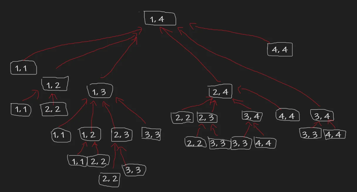
Notice that the leaves of our tree are all the sub-segments of length 1. Imagine visually pruning all the leaves from our tree. We will now have a new set of leaves.

These are the new states/sub-problems to calculate. Notice that after performing such an operation, we have a mix of segments of different lengths. But which ones can be computed completely after having just computed the previous leaf states?

Notice that these are just the segments of length 2. $[1, 2], [2, 3], [3, 4]$. We can perform this operation again, and again, and so on till we reach $[1, 4]$. In general, this construction can be extended to any general $[1, n]$.

From this, it is easy to realize that we are computing DP states in order of increasing the length of sub-segments. Our DAG would look as follows.

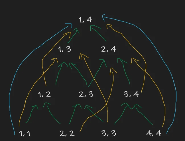
Here, I’ve attempted to paint the arrows showing the transition from a state of length just 1 below in green, 2 below in yellow, and 3 below in blue.

There are no cycles and we have $O(n^2)$ nodes.

DP ≠ Shortest Path on DAG

While the shortest / longest path in a DAG example was quite useful to visualize DP previously, we must realize that this is not always the case. Why?

This is because the state at some node $[i, j]$ is not just dependent on the previous state. Remember that there is a cost associated with every multiplication that is dependent on the state it is being compared with.

For example, when computing the solution at node $[1, 3]$, it is not enough to just consider the cost from $[1, 1]$. The cost at $[1, 3]$ only has meaning when we sum up the total effect from both $[1, 1]$ AND $[2, 3]$.

In this DP solution, we cannot simply construct a DAG structure and find the longest/shortest path as the solution for that node is reliant on the values of multiple nodes. It was a great way to visualize and be introduced to DP, but it is not always the case :)

Can we do better?

Last time, we were able to reduce the space complexity of our DP by realizing that the DP only relied on the states of the DP solution exactly one level below the current level. However, here we realize that this is sadly not the case. The solution at some node $[i, j]$ is very much reliant on every level below it. 1D row optimization etc does not seem to be of much use here. There is also no monotonicity that can be exploited to make the linear computation at some node logarithmic similar to how we did with LIS. Hence I do not think there is a better way to solve this problem.

References

These notes are old and I did not rigorously horde references back then. If some part of this content is your’s or you know where it’s from then do reach out to me and I’ll update it.

1. Professor Kannan Srinathan’s course on Algorithm Analysis & Design in IIIT-H