Preface & References

I document topics I’ve discovered and my exploration of these topics while following the course, Algorithms for DNA Sequencing, by John Hopkins University on Coursera. The course is taken by two instructors Ben Langmead and Jacob Pritt.

We will study the fundamental ideas, techniques, and data structures needed to analyze DNA sequencing data. In order to put these and related concepts into practice, we will combine what we learn with our programming expertise. Real genome sequences and real sequencing data will be used in our study. We will use Boyer-Moore to enhance naïve precise matching. We then learn indexing, preprocessing, grouping and ordering in indexing, K-mers, k-mer indices and to solve the approximate matching problem. Finally, we will discuss solving the alignment problem and explore interesting topics such as De Brujin Graphs, Eulerian walks and the Shortest common super-string problem.

Along the way, I document content I’ve read about while exploring related topics such as suffix string structures and relations to my research work on the STAR aligner.

DNA Sequencing

DNA sequencing is a powerful tool used by scientists to study topics such as rare genetic diseases in children, tumors, microbes that live in us, etc. all of which have profound implications on our lives. Sequencing is used pretty much everywhere in live sciences and medicines today. The technology used for sequencing has come down in cost and that has caused for a big ‘boom’ in the development of this field, similar to how transistor prices going down kick-started the computing industry.

Algorithms play a key role in this field. Take for example, the effort to sequence the human genome back in the late 90s. There were two popular school’s of thought, one who believed that an algorithm crux to the sequencing of the human genome (called de novo assembly) was computationally infeasible in practice, while the others believed that with a large enough compute node it was indeed possible. Finally, it was the second set of people who succeeded by tackling the computational challenge head to head, which allowed them to progress much quicker. It is important for us to know what’s possible and what’s practical to actually compute. Further, knowing about what work has already been done is the first step to figuring out where the next contribution’s should be and how.

DNA sequencing: Past and present

First generation DNA sequencing was a method invented by Fred Sagner and was also known as “Chain termination” sequencing. It was quite labour intensive but over the years improved and many tasks were automated. The HGP (Human Genome Project) used 100s of first generation DNA sequencers to sequence the human genome. However, what we’re more interested in is what happened to the cost-per-genome ratio right after the end of the Human Genome Project towards the beginning of the 2000s.

Source: Sequencing Human Genome Cost - NIH

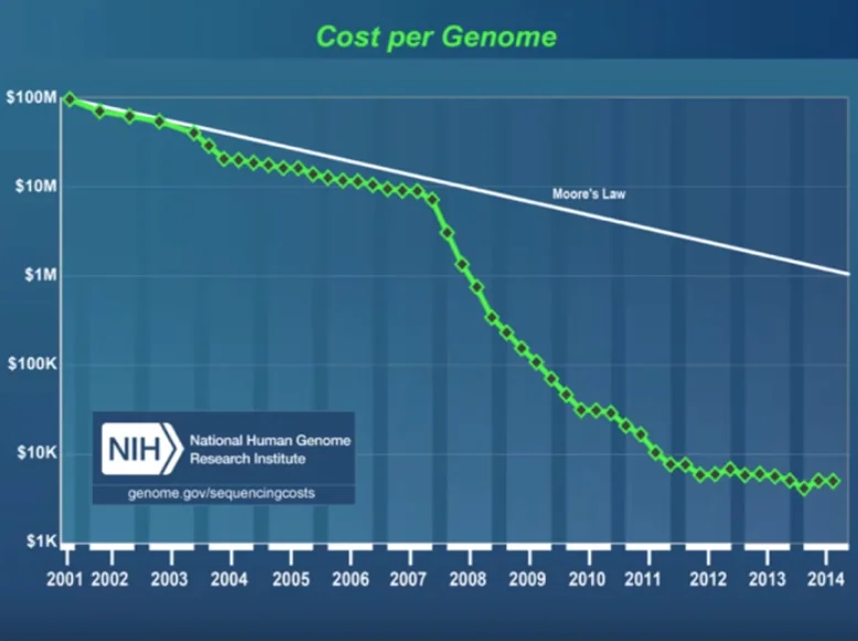
As we can see, something important happened around the year 2007. This is the year when a new kind of sequencing technology started to be used in life science labs around the world. This technology was called ’next’ generation sequencing or ‘second’ generation sequencing. But the name that probably describes it best is ‘massively-parallel’ sequencing. Add to this improvements in technology, speed, etc. and there was massive technological and algorithmic improvements in this field since then.

How DNA Gets Copied

DNA as Strings

We are pretty familiar with the double-helix structure of DNA. If we un-ravel this helix and just pick one of the two ‘rails’, then this strand of the original DNA sequence is split into four sub-sequences made up of the bases A, C, G, or T so that four point sets may be created based on the position of each nucleotide in the original DNA sequence in order to fully use the global information of the DNA sequence. This means that we can represent DNA sequences in the form of a long string containing just the characters ‘A’, ‘C’, ‘G’ and ‘T’.

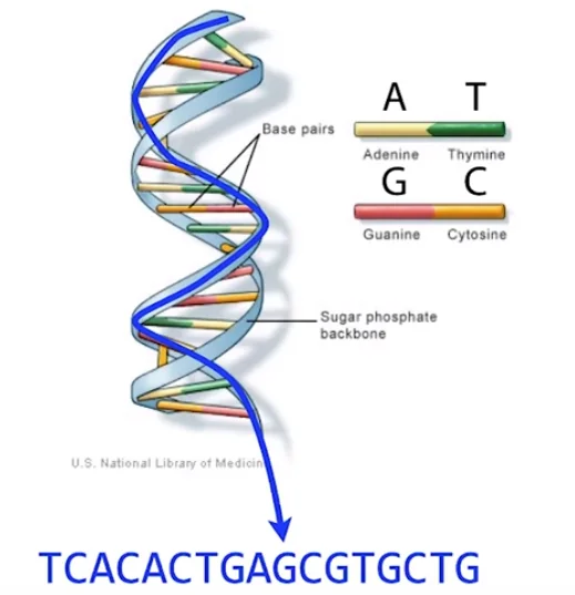
This has further implications that any read of the DNA sequence simply translates to sub-strings in the original DNA string. This essentially allows us to use the massive literature and work that we have done in the field of string algorithms in the field of DNA sequencing.

The copying process

DNA exists in base pairs A-T and C-G. Your genome is almost present in every cell in your body, therefore when one of these cells splits, it must transmit a copy of your genome to each of the progeny cells. Consequently, DNA is first double stranded before being divided into two single stranded molecules. It seems as though we split this ladder straight down the middle. We now have two distinct strands as a result of the separation of the complimentary base pairs. The genome sequence is still recorded on each strand, and the two strands are complementary to one another despite their separation. It acts as a sort of template and provides the instructions necessary for re-creating the original DNA sequence. The name of the molecule, the enzyme that puts the complementary bases in it’s place, is called DNA polymerase. Given one of these single-stranded templates and a base, DNA polymerase is a tiny biological device that can synthesize DNA (this base might be floating around somewhere just waiting to be incorporated). With these two elements, the polymerase will piecemeal construct the complementary strand to produce a double-stranded replica of the template strand.

Massively parallel DNA sequencers

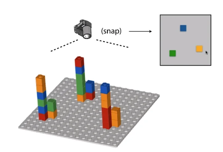
Reads refer to random sub-strings picked from a DNA sequence. One human chromosome is on the order 1 million bases long. Massively parallel sequencers produce reads that are around 100-150 bases long, but produce a huge amount of them. A sequencer ’eavesdrops’ on the DNA copying process to sequence many templates simultaneously. This is how the process works in a nutshell.

1. Convert input DNA into short single-stranded templates.

2. Deposit on slide (scattering the multiple strands randomly across surface)

3. Add DNA polymerase to this slide

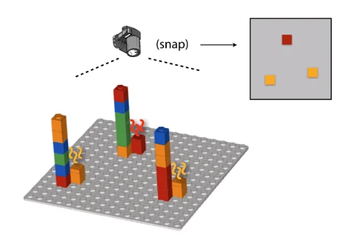
4. Add bases (raw material) to this slide, which are ’terminated’ by a special chemical piece which doesn’t allow the polymerase to construct anything on top of the base it adds to the template.

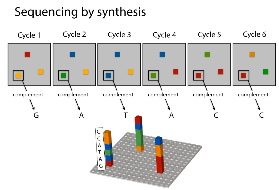
5. Take a ’top-down’ snapshot of the entire slide. (Terminators are engineered to glow a certain color which allows easy identification of the base)

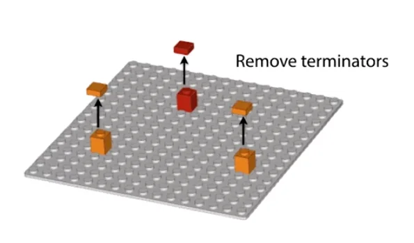
6. Remove the terminators

7. Repeat until all the templates are built fully

The following is a visual depiction of the same.

Sequencing Errors and Base Quality

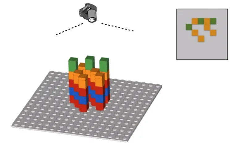
The process described above is largely accurate, but a minor detail we skimped out on is that before the sequencing begins, we amplify each template strand with multiple copies in a cluster. This allows the camera to more easily spot the glowing color of each cluster as just one strand is not enough to accurately distinguish the color. However, there is a hidden problem here. Say during one of the build cycles one of the bases in the solution is unterminated. This would cause the polymerase to go ahead and place the next base as well on top of what should’ve been this cycle’s base. Now because this is a cluster, the majority color would still likely dominate. However, notice that once a base is out of cycle, it will always remain out of cycle. This means that with more and more cycles, the rate of error gets higher and higher.

To counter this, we developed software called the ‘base caller’ which analyzer the images and tries to attach a confidence score to how confident it is about the base for each cluster in each cycle. The value reported is called the ‘base quality.’

$p$ is the probability that the base call is incorrect. This scale provides an easier interpretation of the probability value. For example, $Q = 10 \to 1$ in $10$ chance that the call is incorrect. $Q = 20 \to 1$ in $100$, and so on. The probability computation probably involves ML model nowadays but a reasonable measure one would imagine is simply computing

if it predicts orange as the base.

Re-Constructing Genome Using the Sequencing Reads

Once we have the billions of tiny sequenced reads, they are analogous to having a lot of tiny paper cutouts of a newspaper. Good for a collage, but not useful for reading the news. To make sense of these reads, we need to be able to stitch this back into one complete picture (back to the genome). To do this, we consider the following two cases.

• When there already exists a genome reconstruction of the same species

• When there exists no such reconstruction. (We are sequencing a new exotic species.)

Case I

We rely on the fact that the genomes of two different animals of the same species have $\gt 99 \%$ similarity in their genomes. That is, if we already have a sequenced genome from the same species, we can be guaranteed that the new genome will be extremely similar to the already reconstructed genome. If we imagine genome reconstruction similar to putting together a jigsaw puzzle, the already existing genome reconstruction is something like a photograph of the completed puzzle. We can then rely on this existing construction to guide us in putting together the jigsaw.

In our context, what we can do is match these short reads to the original sequence and see which places in the original sequence are very good matches for our read. We then use these markings as a guide to where the short read actually fits in the puzzle of the complete genome reconstruction. However, as we see in one of the practice labs, simply doing exact string matching is not sufficient. In practice, we find that trying to find exact matches of the short read in the original sequence gives very low matches in the original sequence. In the context of reconstructing our puzzle, this means we have very few clues to go off of for reconstruction. This happens primarily due to two main reasons:

1. The DNA sequencing process can have errors as mentioned above. Perfect reads are not very likely.

2. The ‘snapshot’ we are following will not be an exact match and will have some (albeit few) differences.

But the primary reason exact matching fails is due to the error(s) inherent in the DNA sequencing process. This essentially gives us a fair idea why exact string matching won’t be sufficient for solving our problem. We later explore approximate matching and alignment problems which are primarily what we use to tackle this issue. (Algorithms for Approximate String Matching - Alignment, Booyer-Moore & Knuth-Morris-Pratt for Exact Matching).

Case II

In the case where there exists no already existing snapshot to follow, we will have to tackle the same problem faced by the people working on the original Human Genome Project (HGP). We rely on techniques of de novo assembly to reconstruct the genome string. We will discuss this in more detail towards the end of the course.