Branch & Bound

When trying to solve problems in general, (especially optimization problems) it’s always a good idea to formulate a mathematical definition of the problem. To formulate it in mathematical terms, we assign each item in the knapsack a decision variable $x_i \in \{0, 1\}$. Now, each item in the knapsack also has some weight $w_i$ and value $v_i$ associated with it. Let’s say our knapsack capacity is denoted by $W$.

The decision variable $x_i$ simply indicates whether we include item $i$ in the knapsack or not. Using this, we can define the objective function that we wish to optimize (maximize) as:

Under the constraints that

Now we have a formal definition of the function we want to maximize under some constraints.

Branching

Now, one way to solve the knapsack problem would be to perform an “exhaustive” search on the decision variables. This would mean checking every possible combination of values that our decision variables could take. Visualized as a tree, it would look like this:

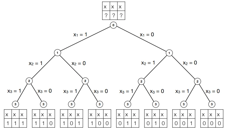
Here, we compute the answer by branching over all possible combinations. This is, of course, $O(2^n)$. Increasing input size by one would literally mean doubling the amount of computation done.

Relaxation

This is where the idea of relaxation comes in. Branching was basically us splitting the problem down into subproblems by locking or constraining each variable and then deciding on the constraints for other variables. Exhaustive search isn’t ideal, hence we try to reduce the search space by implementing some “bound.” Essentially, at each step of the recursion, we place an optimistic bet or estimate on just how good the solution to our subproblem can be. If at any point in the recursion, this estimate is lower than the best-found value so far, we can kill off the recursion.

As we’ve mentioned before, relaxation is the key to optimization. The original problem is NP-Complete. This means that until someone can prove $P=NP$, these problems have NO polynomial-time optimal solution. Relaxation is the art of how we deal with these problems.

Using relaxation on the exhaustive search

So, what constraints can we try to “relax” in the knapsack problem? The only constraint there is the weight of the Knapsack. So let’s start by relaxing it to let us have an infinite knapsack. A picture is worth a thousand words, so let me just show you what the search would like with this relaxation.

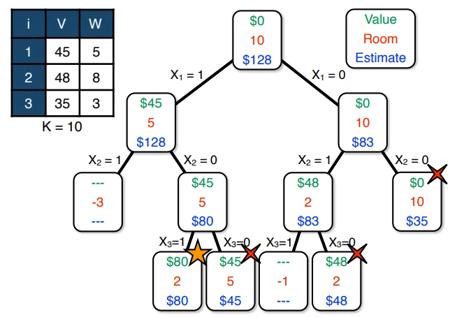
Let’s try to see what we did here. First, we begin by letting root have $W = 10$ space and have $V = 0$ as it is completely unfilled. This is the $(0, 0, 0)$ state. The estimate here is our relaxation. Assuming infinite space, we see that the most optimistic value we can reach from here is $\$128$ if we include all the items. Remember, the relaxation is for calculating this estimate.

Once this is done, we’re just performing an exhaustive search. But now, notice that the node on the left stops its recursion once the room in the knapsack has become negative. This is a simple base case on the original recursion.

The interesting part is the recursion that we’ve killed on the rightmost node. The leaves marked with crosses went till the end until they were discarded in favor of the left bottom leaf which is our optimal score of 80. Now, the rightmost node was killed even before it reached the leaves. This is because we had already achieved a better score (80) than the best possible estimate from this node. Hence we know for a fact that following the recursion can never give us a better score. Recall that our relaxation was an infinite knapsack. If we cannot do better with an infinite knapsack from that point, there is no point in searching further down that track. This is the key idea behind relaxation and how using bounds can help us optimize exhaustive search. However, this particular relaxation was not very effective and did not help much in optimizing our search. But maybe with a better heuristic, we can optimize the search further.

Coming up with a better heuristic

Let’s think about how we would normally solve the Knapsack problem if we were allowed to take rational amounts of an item. That is, it is no longer a 0-1 problem where we must either take or discard an item. We can take items in parts now. This problem has a fairly straightforward and greedy solution. We simply sort items by $\frac{v_i}{w_i}$. This is essentially their “value per 1 unit room.” Simply pick the element that gives the best value per weight. So the strategy is now picking the element with the highest $\frac{v_i}{w_i}$ ratio, and when we run out of space pick the last element in a fractional amount such that it fills up the entire knapsack.

This is the optimal solution for this version of the knapsack problem. But what about when we apply this relaxation to the original exhaustive search model instead of the infinite bag relaxation?

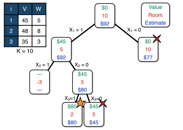
Notice how much better we’ve managed to optimize the exhaustive search. The right child of the parent node is cut off at $\$77$ and does not search further, because our "estimated" cost is lesser than the highest value we have found so far ($$80)$.

Optimality

Notice that the fractional knapsack is the best-case version of the knapsack as we can optimally fill every unit of space according to a greedy strategy. Therefore if even the greedy estimation is below previously found maxima, then this quantity cannot be optimal. This means this branch and bound relaxation will still give us the optimal solution to the 0-1 knapsack problem.

Complexity

Analyzing the running complexity of branch and bound algorithms has proved notoriously difficult. The following blog gives some intuition as to why we find placing a bound on such techniques very difficult. https://rjlipton.wpcomstaging.com/2012/12/19/branch-and-bound-why-does-it-work/

George Nemhauser is one of the world’s experts on all things having to do with large-scale optimization problems. He has received countless honors for his brilliant work, including membership in the National Academy of Engineering, the John Von Neumann Theory Prize, the Khachiyan Prize, and the Lanchester Prize. To quote him,

“I have always wanted to prove a lower bound about the behavior of branch and bound, but I never could.” - George Nemhauser

Putting a good bound on branching and bounding is very difficult and is an open problem. One alternative measure that is used to better estimate the efficiency of branch and bound algorithms is its effective branching factor (EBF).

We define EBF as the number $b$ so that your search took the same time as searching a $b$-ary tree with no pruning. If you are searching a tree of depth {d}, this is well-defined as the $d$-th root of the total number of nodes you searched.

This is computed in practice and is used a lot in solving optimization problems as it is quite effective in practice, even if it is difficult to put bounds on theoretically. The fact that the runtime can be altered significantly by simply changing the relaxation criteria also makes it a great option to try out when coming up with relaxation ideas.

Why not just stick with Dynamic programming?

This is a natural question. (A Deep Dive into the Knapsack Problem) DP seems to give us an approach where we can be comfortable in sticking with an $N_W$ or $N_V$ complexity solution. However, what if we modify the question ever so slightly and allow items to have fractional or real weights? This seems like a problem that might surface in the real world a fair amount. The DP table approach is no longer feasible. In such a situation the branch and bound algorithm might come in clutch. As we explore such problems and minor variations of such problems, the need to expand our tool-belt and come up with more and more optimization algorithms becomes clear.

References

These notes are old and I did not rigorously horde references back then. If some part of this content is your’s or you know where it’s from then do reach out to me and I’ll update it.

1. Discrete Optimization - University of Melbourne - Coursera