Previously, we looked at a few famous dynamic programming problems (DP as DAGs, Shortest path on DAGs & LIS in O(nlogn)). Today we’ll be looking at a pretty common problem that we have our computers solve for us, almost every single day. Spellchecking. Our computers are great at suggesting good auto-correct solutions for us whenever we misspell something. But to recommend one choice over the others, there must be some measure of ranking them. The problem is as follows:

The problem

Given two strings X & Y, what is the minimum number of edit operations that we must perform on X to transform it to Y? Here, an edit operation can be one of three things.

1. Insert character $c$ at any position $i$ in $X$
2. Delete character $c$ at any position $i$ in $X$
3. Substitute character $c$ at position $i$ in $X$ with any other character $c'$

This computed quantity is also known as the Levenshtein edit distance between the two strings.

In essence, the Levenshtein distance is a very good heuristic to measure just how close two strings really are. It’s a very good metric to rank words that the user might’ve wanted to type but accidentally misspelled due to one of the three possible edits. It is understandable why this is often used for spellchecking.

An alternate view

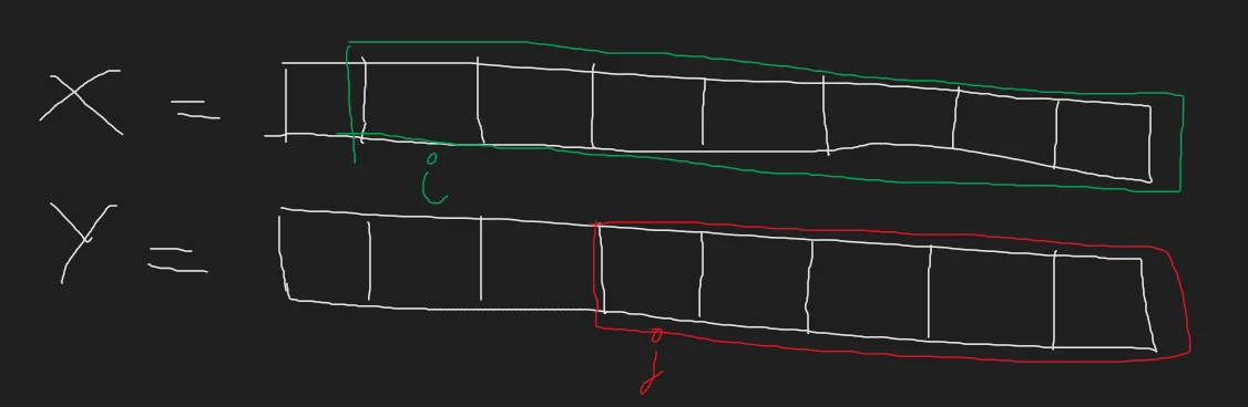
Another way to think about edit distance is as an alignment problem. Given two strings $X$ and $Y$, to what extent can they be matched up? An example should make this question more clear.

Notice that with this alignment,

1. The _ ’s in $X$ represents an insertion edit
2. The _ ’s in $Y$ represents a delete edit
3. And a character mismatch represents a replacement edit.

At position 2, we have an insertion edit $(\_, U)$. At position 4 we have a replacement edit $(O, N)$. At position 5 we have a delete edit $(W, \_)$. This is in fact the optimal answer, and hence, the Levenshtein distance between the two strings.

In short, if we look at it as an alignment problem, the cost is the number of mismatched columns. The edit distance would then be the best possible alignment which minimizes mismatches.

Finding a recursive solution

At first glance, finding the solution to this question seems very difficult. There are a lot of different ways to convert say “Dinosaur” to “Paragraph.” It is not very clear how to solve this question without brute-forcing a lot of pairs. However, a key insight we can make here is that once we have optimally matched some prefix or suffix, we can discard away the matching prefix or suffix and recursively solve for the rest of the string.

An example will help illustrate this point. Consider the strings “Dog” & “Dinosaur”. What the above point means is that the Levenshtein distance between Dog & Dinosaur will be the same as the Levenshtein distance between “og” & “inosaur”. This key observation lets us write a nice recursive algorithm to calculate the Levenshtein distance for two strings.

The algorithm

The top three cases are the base cases. If $Y$ is empty, we have to delete every character in $X$. If $X$ is empty, we have to insert every character in $Y$ in $X$. There is no other way to optimally transform $X$ to $Y$.

The third case is the key point discussed above. If the first characters match, we can simply discard it and compute the answer for the rest of the string.

If none of the above cases are true, we can do any of the three edit operations. Notice that there is sadly no way of greedily picking what the best option would be here. Every operation influences the alignment of the rest of the substring and it is not possible to determine how a local choice affects the global structure we end up with. Hence the only possibility here is to recursively try out every possible combination and pick whichever gives us the minimum. Notice that each of the cases corresponds with an edit operation.

1. $Lev(tail(X), Y) \implies$Insertion operation. We are inserting a _ in $X$ and computing the answer on the rest of the string.
2. $Lev(X, tail(Y)) \implies$Delete operation. We are inserting a _ in $Y$ and computing the answer for the rest of the string.
3. $Lev(tail(X), tail(Y)) \implies$Replacement operation. We are substituting the character. This corresponds to letting the mismatch exist and align the rest of the string.

Optimum substructure exists!

This algorithm has exponential complexity because in the worst case, it is trying out three different operations at every step. But the good thing about defining this problem recursively is that we have found an optimum substructure for this problem. If we brute force all possibilities at some position $i, j$ in both the strings, we can discard this character and recursively solve on the suffix. This hints us towards using DP to solve our problem more efficiently.

Coming up with a DP solution

In general, when we try to find a DP solution to some problem, the following is a good mental checklist to follow/answer.

1. Define the subproblem & count how many we’ll have
2. Guess some part of the solution & count how many possibilities we’ll have to brute force over. This is the transition we want from the problem to its subproblem.
3. Write the recurrence in terms of the guessed solution + the subproblem
4. Figure out how to memoize/use a dp table for storing computed calculations. Notice that the recursive structure must follow a DAG structure as stated previously or we’ll have an infinite recursion which implies our algorithm is wrong.
5. We solve the problem

Let’s go over them one by one.

Looking at the recursive definition we have for edit distance, it becomes clear that we must be able to compute the edit distance between any two prefixes of string $X$ and $Y$. These are all the different subproblems encapsulated by the recursion.

Note, from here on forth we denote prefixes of $X$ by $[\ :i]$ and prefixes of $Y$ by $[ \ :j]$. Here, we get the answer to the first point in our checklist.

1. Computing edit distance for all possible pairings of prefixes between $X$ and $Y$. We will have of the order quadratic subproblems. For every value of $i$ we have $j$ possibilities to pair it with. Hence the number of problems is of the order $O(|X|.|Y|)$

For computing the answer at every point, we either have the base case or we have three possible operations to take.

1. We can perform one of three operations. Substitute, insert, or delete. In essence, given two suffixes we have exactly three operations that we can use to transform the first character of $X$ to the first character of $Y$. Replace $X[i] \to Y[j]$. Insert $Y[j]$. Delete $X[i]$.

Since we already have a recursive expression of the algorithm, we already know the recurrence.

3. The recurrence is the same as stated previously

1. We already said we will have $O(|X|.|Y|)$ subproblems where we match every $i$ with every $j$. This should have hinted at a 2D dp table. In this table, every cell corresponds to the edit distance computed between two suffixes of strings $X$ and $Y$.

For example, the highlighted yellow cell represents the edit distance between LITY and ARITY. Further, notice that each of the three highlighted boxes around it corresponds to an edit operation. This observation is key to figuring out the topological ordering of our problems.

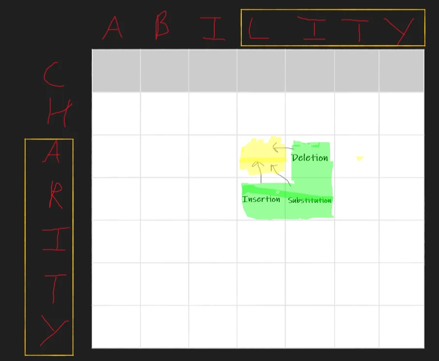
1. The Substituion box means we swap “L” with “A” and move to state $(i+1, j+1)$.
2. The Insertion box means we insert “A” and move to state $(i, j+1)$
3. The Deletion box means we delete “L” and move to state $(i+1, j)$

Hence for computing the answer at any cell, we only need the answers at cells $(i+1, j), (i, j+1) \text{ and } (i+1, j+1)$. This is enough information to get the topological ordering. A simple nested for loop from $i :n \to 0$ and $j:m\to0$ should be sufficient.

Notice that due to the nature of the problem I can go from $0\to n$ and $0 \to m$ as well and define the dp for the prefixes. However, the suffixes idea in my opinion makes the most sense and we’ll be using the suffix definition for the dp.

Further, notice that in the real dp table we would have an extra row and column padding at the very ends to account for the base case where $|X| = 0$ or $|Y| = 0$.

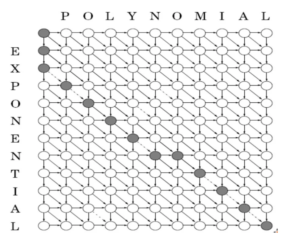
Thus far, we have implicitly assumed that the cost associated with each operation is 0. However, this need not be true. Each operation can have any defined cost. In fact, we can even define the cost for conversion from one specific symbol to another and our algorithm would still work. The above DP table can simply be thought of as a DAG with $O(n^2)$ nodes and each edge $(u, v)$ can be weighted with the cost of the corresponding transformation from the symbol at position $u$ to the symbol at position $v$. Our final answer is in fact just the shortest path from position $(|Y|, |X|) \to (0, 0)$

Visualization as a DAG

Note: This is the image from the lecture slides and shows the path for the approach using prefixes. For the suffix-based state transformation used by me, simply reverse the direction of each edge in the graph and the problem remains the same.

1. Now to solve the problem :) Notice that the runtime of the algorithm is $O(|X|.|Y|)$

Single row optimization

The time complexity of our algorithm was $O(|X|.|Y|)$ and the space complexity was also $O(|X|.|Y|)$. This is considerably better than exponential, but can we do better?

Are there any redundancies that we may be computing/storing? It turns out that in fact, there is.

Notice that to compute the value of $dp[i][j]$ at any location, we only care about the values of $dp[i][j+1]$, $dp[i+1][j]$ and $dp[i+1][j+1]$. However, notice that we are storing the ENTIRE dp table from $dp[0][0] \to dp[n][m]$. This is redundant and can have great practical limitations on our algorithm.

For example, computing the edit distance between two strings of length $10^4$ would require 100 MB of memory. This in turn would give a lot of cache misses and slow down the algorithm as well. Further, if we wanted to compute the distance between a string of length $10^5$ and $10^4$, it would only take a few seconds to a minute on most machines but it would require 1 GB memory.

That’s a lot of memory wasted for storing redundant information. The single row optimization for DP is as follows.

We only ever store two rows in our DP table. When computing $dp[i][j]$, we only store the dp table at row $dp[i]$ which we are computing, and the row $dp[i+1]$, which contains the already computed values (as enforced by the topological ordering).

Notice that with this simple optimization,

1. To compute any $dp[i][j]$, notice that all the required states are always in memory. We are never losing/erasing dp values that we require for the computation of $dp[i][j]$ before computing $dp[i][j]$.
2. We have reduced the space complexity of our algorithm from $O(|X|.|Y|)$ which is quadratic, to $O(2*|X|) = O(|X|)$. Our space complexity is now linear!

Applications

While we only discussed how Levenshtein distance was a great heuristic for spell checkers, it is also extensively used in the field of biology for comparing DNA sequences. The more general version where each transformation is given some cost $c_{transform \ type,\ s1 \to s2}$ is used here.

For example, the mutation $C \to G$ is more common than $C \to A$.

Notice that we can now give $C \to G$ a low cost and $C \to A$ a high cost. This represents that the first mutation is more likely than the other. This gives us a measure of how similar two DNA sequences are. Mutations also have insertions/deletions. This makes Levenshtein distance a great tool to use here.

If we wish to not use insertions or deletions, notice that we can simply give them $\infty$ cost. In computational terms, they’re given a very high value like

Code

While it is much easier to visualize the bottom-up dp as finding the solution to suffixes, it is much easier to code the prefix definition of the dp. Note that there really isn’t any difference in which direction we pick, at least not conceptually. It is just easier to implement the prefix solution in code.

The single row optimized dp code for calculating the Levenshtein distance between two strings can be found here: Levenshtein Edit Distance

References

These notes are old and I did not rigorously horde references back then. If some part of this content is your’s or you know where it’s from then do reach out to me and I’ll update it.

1. Professor Kannan Srinathan’s course on Algorithm Analysis & Design in IIIT-H
2. How do Spell Checkers work? Levenshtein Edit Distance - Creel (Excellent channel, do check him out. Has a lot of unique amazing content!)