Just to preface this, this is not going to be a detailed paper deep dive. Why am I doing this one differently? Mainly because I’m bottlenecked on reading and writing time. I’ve not posted anything in the recent few months because of an overload of things to read about and not enough time to write blogs / notes in. The original The Log-Structured Merge-Tree (LSM-Tree) paper here by Patrick O’Neil, Edward Cheng, Dieter Gawlick & Elizabeth O’Neil is 32 pages long and I’ve not had the chance to more-than-skim it. I don’t want to bottleneck my blogs, so I’ll be starting with a high level set of notes / content I’ve amassed from watching CMU’s #04 - Database Storage: Log-Structured Merge Trees & Tuples (CMU Intro to Database Systems) (Have I mentioned I’m a fan of Andy Pavlo? You should watch his courses now!), some blogs / talks about RocksDB given by folk from Facebook, similar content from folk at PingCap (about it’s use in TiKV) & some experience working with TiDB at Databricks.

What motivated LSM Trees?

Long story short, in terms of real-world performance, writes are a lot more valuable to optimize for than reads. Especially in database applications. Why? Because writes in other databases (that provide SOLID guarantees) often require updating several secondary data-structures like indexes, undo/redo logs and also have to possibly propagate through multiple layers of cache. On the other hand, the world was moving towards SSDs and back then, saving memory update cycles on SSDs was also a key metric to improve. This is however, not so important today because SSDs can usually sustain way more program-erase cycles compared to then. Regardless, lesser write operations does mean increased longevity for SSDs, and probably for HDDs as well (lesser arm movement). Reads on the other hand usually just need to traverse data-structures to find the location to read from disk / buffer pool (cache).

In short, the state of the art B+ tree solutions which are theoretically best for the usual (fetch, insert, delete, range_scan) operations may not be best in practice because of the skew / asymmetry between write heavy & read heavy workloads. We wanted to optimize for write speed & efficiency. And that eventually gave birth to the LSM tree.

What is a LSM Tree? How does it work?

A picture is worth a thousand words, and a video is worth a thousand pictures… I guess? Regardless, would highly recommend watching #04 - Database Storage: Log-Structured Merge Trees & Tuples (CMU Intro to Database Systems), at least from 26:53 - 44:59. It’s a great description of how LSM trees work.

There’s two parts to a LSM tree.

1. The in-memory section
2. The on-disk section

In-Memory

A LSM tree primarily functions as a key-value store. So the main operations it’s seeking to support is PUT / DELETE operations, but we can also do range scans. Let’s start by demoing how PUT works on a LSM tree. The In-memory section is mainly what’s called a mem-table.

Mem-table

The “mem-table” is an in-memory data structure that is a sort-of cache layer & the primary receiver of PUT operations. It can be any BBST (balanced binary search tree) or any other data structure that supports fast ($O(\log(n)))$ insertions, searches & updates. A hash-map also works. We define a constant “limit” for the size of this data structure. Let’s say the limit is $6$. Here’s what the mem-table looks like after 3 insertions,

We just insert the elements as the PUT operations arrive into the BBST. If the same key is updated, say I issued a PUT(key974, val_69), the node containing key974 is updated. No new node would be created. However, once the BBST hits a size of 6, the BBST is converted into an immutable SST (Sorted String Table) and stored to disk.

Here’s the mem-table after 6 insertion operations.

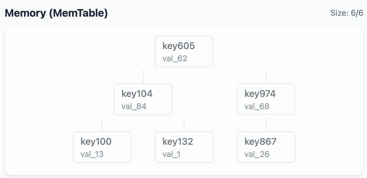
To convert this mem-table to a SST, we do a simple linear-time traversal of this tree to obtain the sorted list of keys:

key100 -> val_13
key104 -> val_84
key132 -> val_1
key605 -> val_62
key974 -> val_68
key867 -> val_26

This structure is called an SST. We now declare this structure immutable. That means, we will not modify this data structure in the future. This SST is then “flushed” to disk to be stored in the “level-0” layer. More on this later.

On-Disk

(Thanks to Claude for helping me generate these images with minimal effort.)

Note: The below is a description / run-through of a level based compaction strategy. There are other compaction strategies (tiered, dynamic, etc.) as well. You can check out RocksDB for descriptions of other compaction strategies and how they compare. We’ll go with leveled here because it’s simple enough and is what the original LevelsDB used.

SSTs

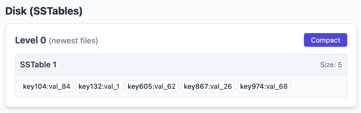
The sorted string tables are stored in what is known as “levels” in LSM-tree speak. What each level contains depends on the ‘compaction’ strategy that the LSM tree uses. For now, let’s just focus on what it looks like on disk. The on-disk representation of our previously full mem-table looks as follows:

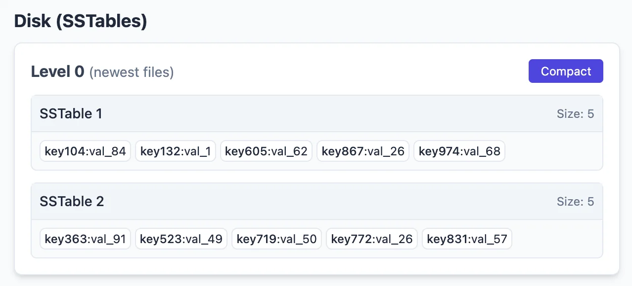
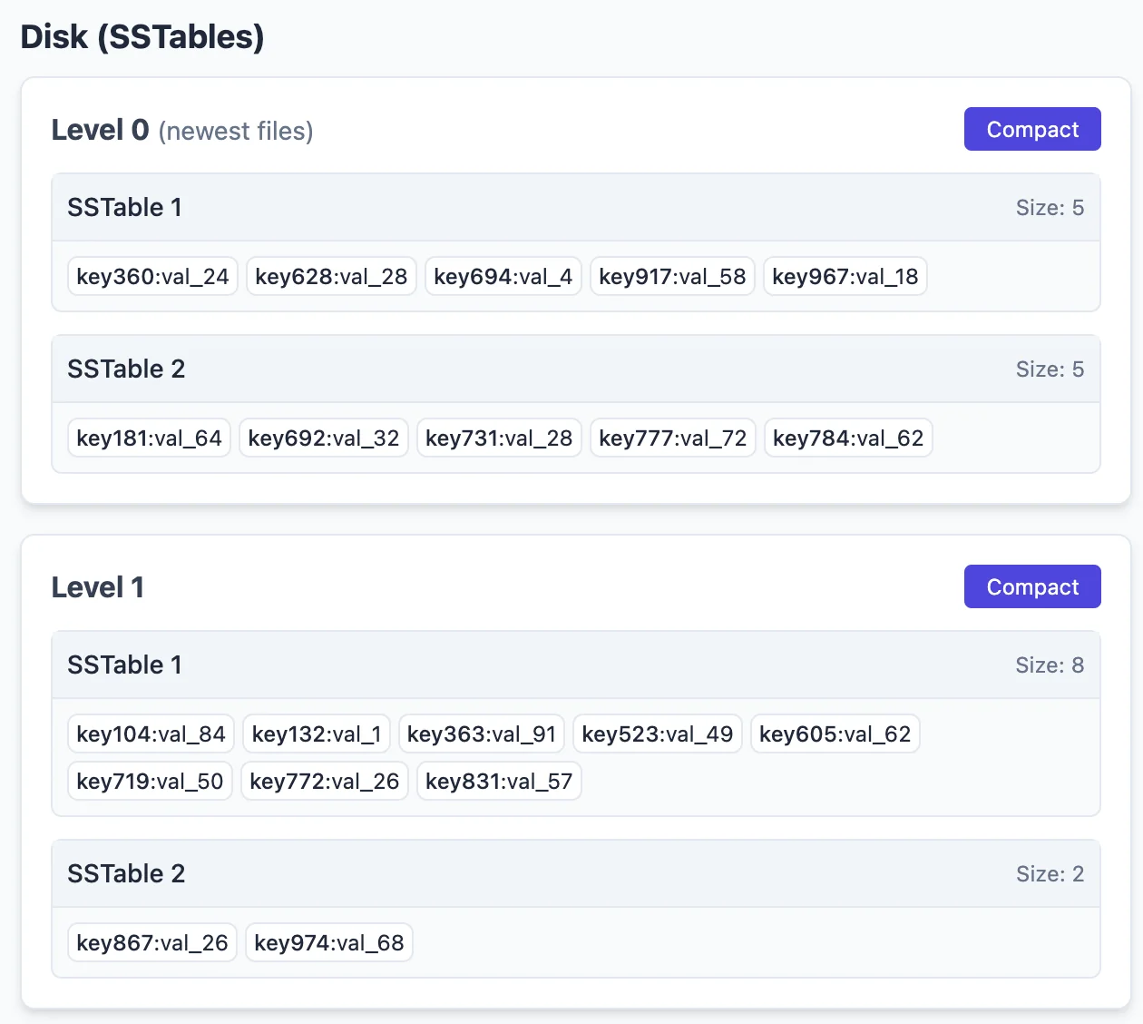
Once I add 6 more records to our LSM tree, the next SST is constructed and flushed to this “level-0” disk storage. Now, we have SSTable 1 & SSTable 2 in our level-0 storage.

And that’s it. Each time a PUT occurs, the new key is added to the mem-table, and the mem-table is periodically flushed to disk as SSTs. Writes are blazing fast because it’s just an insertion into an in-memory, tiny BBST. Pretty much constant. However, reads would suffer a lot because the best we can do is go through every single SSTable on disk and binary search on them. That would be pretty bad.

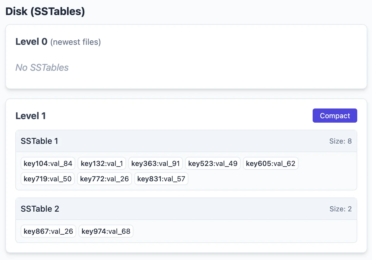
This is where the idea of ‘compaction’ / ‘deferred writes’ comes in and helps change the equation to benefit read performance by allowing asynchronous or deferred write operations. As you can see, the size of Level-0 SSTables are size 5. Let’s say we allow Level-1 SSTables to be as big as 8 in size. We can then asynchronously “merge” two SSTables (in linear time, using logic similar to the merge function in merge_sort) to “compact” 2 level-0 SSTables into a larger level-1 SSTable. For example, if I compacted the above two SSTables, we would get this:

I can insert 12 more new records to let us have 2 new SSTables in level-0 as follows:

Compacting them, gives us:

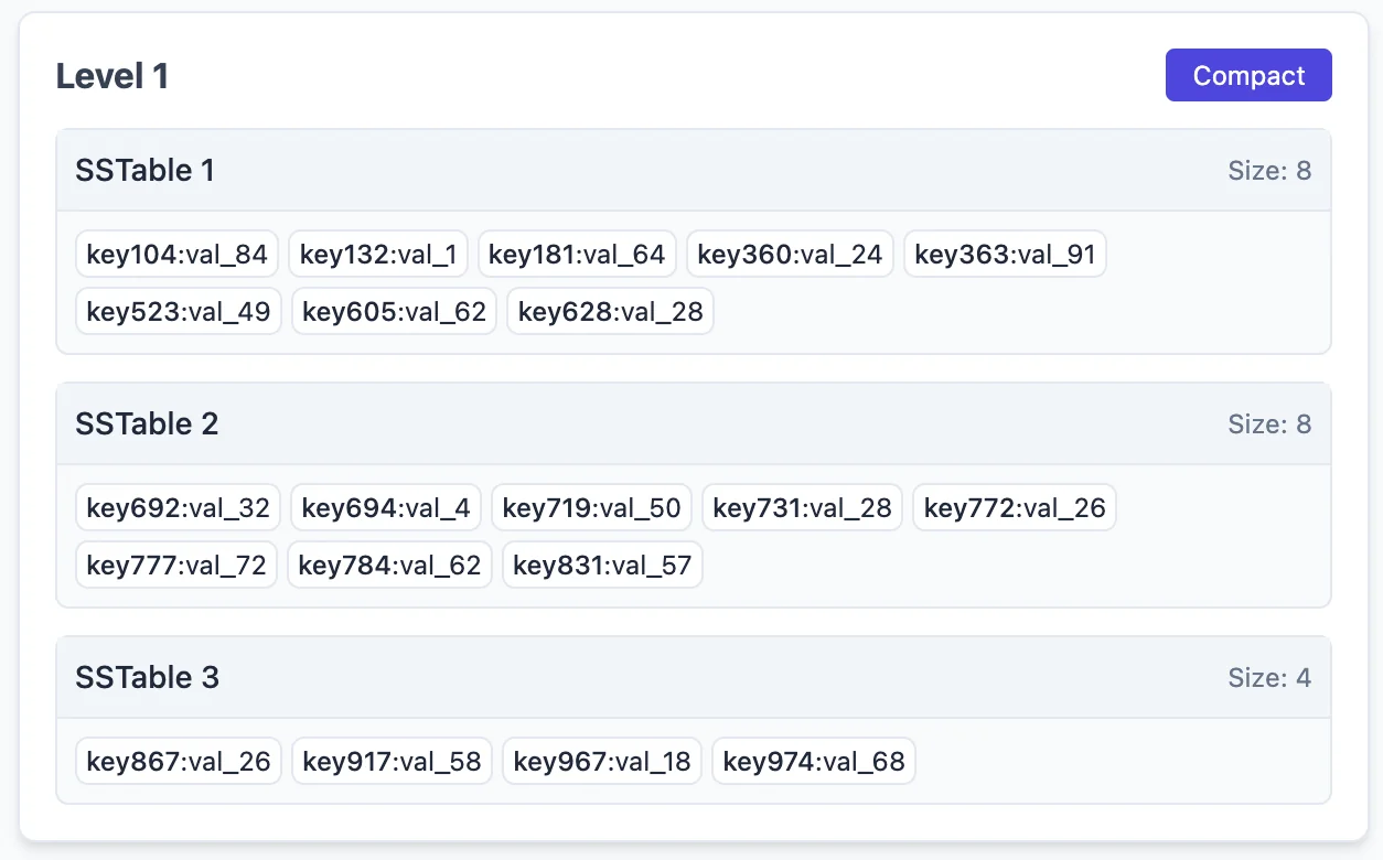
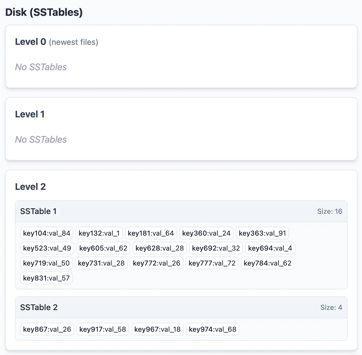
Pay attention to how the SSTables merged. Notice that in level-1, the SSTables are each responsible for disjoint, non-overlapping key ranges. That is, the 2 SSTables in level-0 did not just merge and get shoved into level-1 as new SSTable entries. Corresponding entries in level-1 (both the original level-1 SSTable 1 & 2 entries were deleted, and re-created) were modified and re-written to disk. This is how we choose to compact. Similarly, if we choose to compact the SSTables in level-1, we can combine and push them out to level-2 like so:

Special note about level-0: What I said about each SST being responsible for non-overlapping regions is not true for only level-0. This is mostly an implementation detail, but I believe this is how RocksDB implements it. For Level-0 alone, we just flush the mem-table to disk as is. Earlier entries to the left. When merging some SSTables from level-0, we can use the same merging logic the other layers use (level-0 does not need to be governing disjoint key-spaces). I suggest thinking about it yourself, but the idea is just that the SSTables that need to be affected in the $(i+1)^{th}$ level are still constant regardless of which 2 level-0 SSTs I pick to merge. The only caveat is that level-0 SSTables cannot be binary searched on. Any of the search strategies I describe below implicitly assumes that we do a full linear scan on each of the level-0 SSTs. (We can binary search inside an SST, but I still need to check every SST in level-0). This is mostly a non-issue since level-0 was the mostly recently written to section of disk, which most likely means that the SSTs are in the cache / buffer-pool & very quick to linear search on.

MVCC

Let’s quickly understand the important implications of this kind of a data structure. This data structure implicitly implements MVCC (multi-version concurrency control). Well the concurrency control might not be relevant here, but the point is that multiple ‘versions’ of a key over different instances in time may exist in the data structure. That is, given our current data structure state, if I perform a PUT(key104, val_85) operation, there will be 2 instances of key104 in the data structure. One in level-2, and one in the mem-table. This is fine, because when reading, the version that comes the earliest is the dominant / correct value to read from the data structure.

Similarly, when merging, the version from the higher level overwrites the value of the key in lower levels. We never have trouble working out same-level version problems because we established the invariant during merging that each SSTable in a level is responsible for non-overlapping key spaces.

Point-GET

How do point queries work here? We need to work our way from the mem-table to each of the levels in increasing order. We cannot skip levels because earlier versions of a key are the correct (most up-to-date) ones. If an entry is found in the mem-table, we are done. Otherwise, we have to scan each level one-by-one. To scan any level $i \ (i \gt 0)$, we can exploit the property that each SST is responsible for non-overlapping sections of the key space. That is, we can binary search on the SSTables in each level to find the only (if one exists) SST that is capable of containing the key.

To facilitate this binary search, each “level” of a LSM tree contains some metadata in a ‘summary table’ that contains the minimum & maximum key each SSTable in the level is responsible for. These metadata values can be on-the-fly updated in $O(1)$ during the merge operations.

Remember that in the worst case (the key does not exist in the LSM tree), we still need to go through every level. So in the worst case, for each level we perform one binary search to find the right SSTable to look at then perform a binary search on that SSTable to find the key (if it exists). However, we can do even better, but we’ll get to this in a later section.

Range-GET

I said we can support range scans too. But how? Let’s reason out how we can do range scans on LSM. First things first, defining hard constraints. We have to check every level. Just one of the keys in the range we’re scanning might’ve been written a long time ago and might have been compacted down to the last layer. So we have to scan every layer.

The first obvious idea might be to:

1. Binary search the lower bound for the key in each range to identify the first valid key in a level in logarithmic time
2. Aggregate all the valid keys for each level one by one
3. Merge sort the final results
4. Send them back to the client

This would work, but it’s pretty inefficient since we need to aggregate and merge possibly lots and lots of keys. (What about a range scan for the whole table?)

Instead, we can use a more online / streaming method. Consider the following picture as the current state of our mem-table, and we are trying to stream the results for a RANGE_SCAN(key640, key694). I’m going to assume level-0 is sorted here for simplicity, in practice, level-0 would need some aggregation logic.

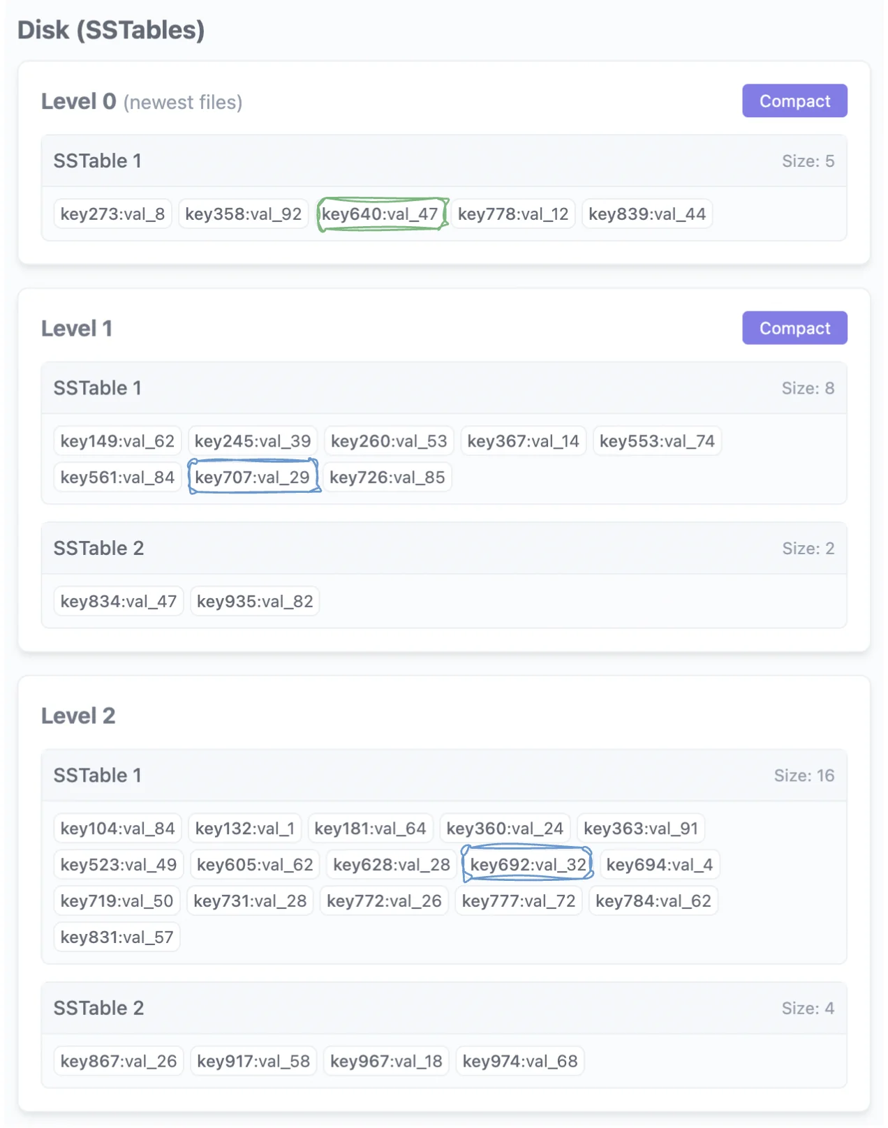
The results of our binary search identify the highlighted three keys across each level. key640 from level-0, key707 from level-1 & key692 from level-2. Now, how can we avoid aggregating results for each run and merging them offline? We need to make our queries work online but without much space / time overhead. What properties can we use here? Let’s assume each insertion was an unique key first.

1. Note that in each range, advancing the ‘iterator’ to the currently highlighted cell will always give us a key that is greater than the currently highlighted key
2. This means that the first valid key in our range scan will always be the minimum value among the highlighted cells (in this case, key640).
3. Let’s denote $key^{L}_{\geq k(i)}$ as the first key record in level $L$ that is greater than or equal to the key value of the $i^{th}$ record. Then we can see that, in fact, after some record $i$ is streamed back to the client, the next record to stream back will always be the $\min(key^{L}_{\geq k(i)})_{\forall L}$.
4. Remember our iterators in the above diagram? We define that our iterators will always be present at position $key^{L}_{\geq k(i)}$ after the streaming of record $i$. Is this easy to maintain?
5. Yes, once key640 is streamed, just move the iterator by 1 to key778 in level-0. Remember that we always stream the $\min(key^{L}_{\geq k(i)})_{\forall L}$ key. This key must belong to some level $L$. We can then always move the iterator by 1 to the next key in this level, and this key must be the $key^{L}_{\geq k(i)}$ for that level because the previous record streamed was $k(i)$ and by definition, this key is the next greater element in that level.

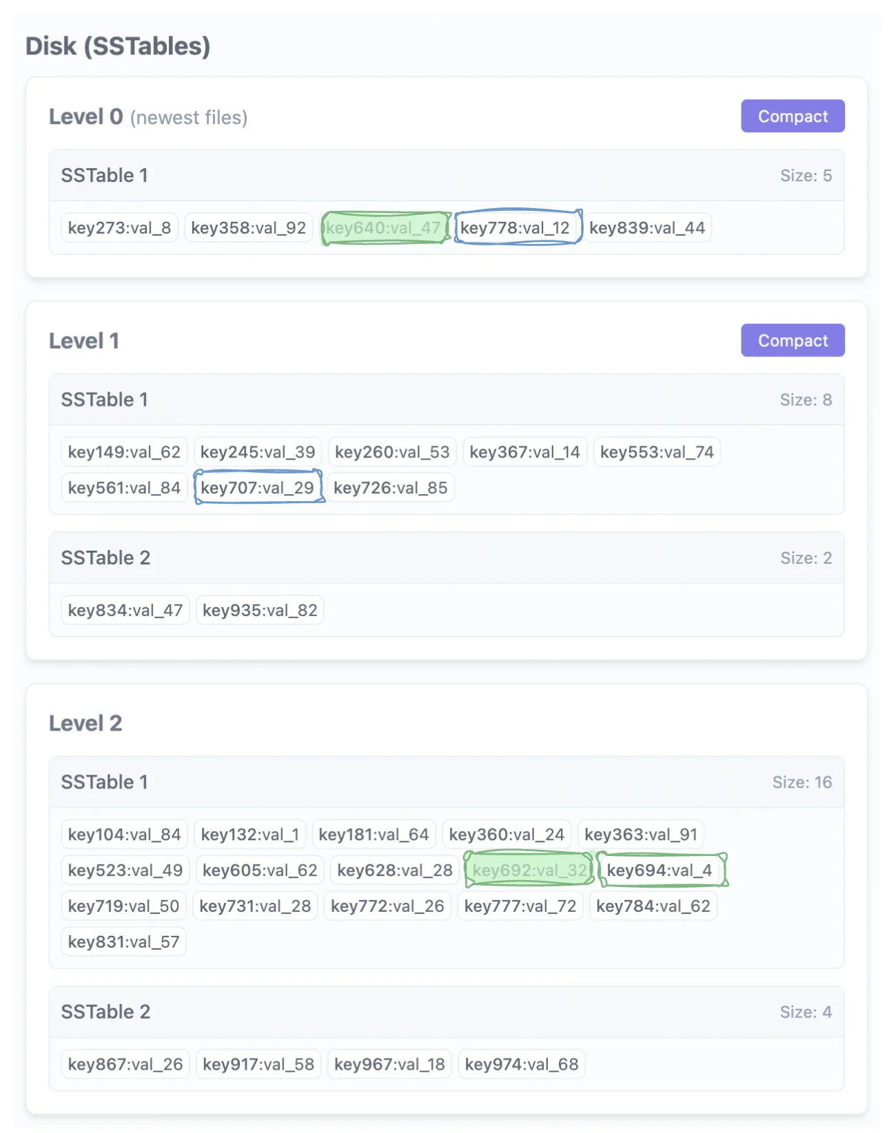
So back to our diagram, taking the min over the values again, we would see that the next key to be streamed is key692:

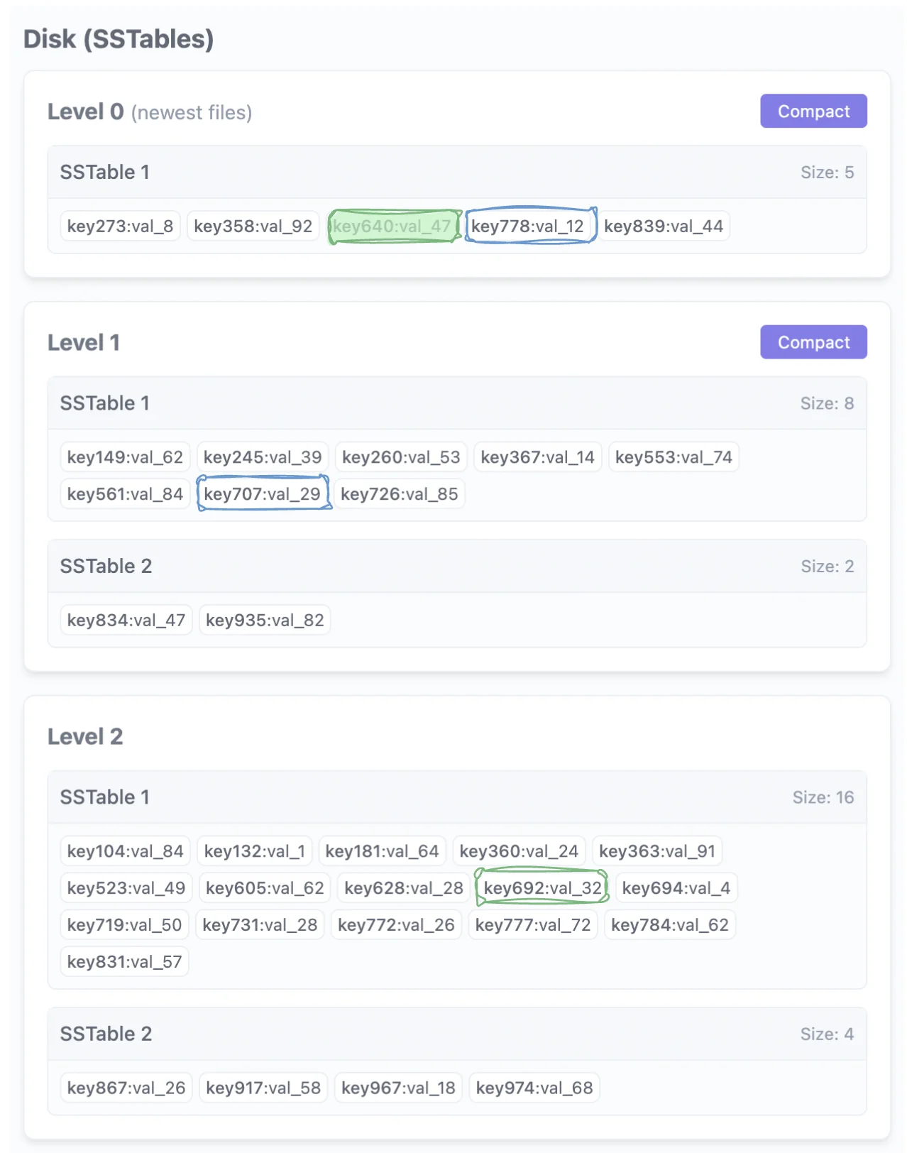
Let’s stream it and move the iterator forward. Taking the min again, we stream key694. After that, all the keys are greater than the $R$ of our query range $[L, R]$. So we are done.

Also see FAST ‘21 - REMIX: Efficient Range Query for LSM-trees for more ideas / follow up reading (or watching).

What about multi-versioning?

Fair question. Does this still work if key inserts aren’t unique? What if a key $x$ exists in $level_i$ first and then also in some $level_{j \gt i}$? To handle multiple versions, we only need to tweak our comparator slightly. When streaming back the next record, the problem is a conflict in resolving the expression $\min(key^{L}_{\geq k(i)})\forall L$ because there might now be multiple equal values of $key^{L}_{\geq k(i)}$ for the same level. We just change the comparator to sort by $(key^{L}_{\geq k(i)}, L)$ instead. That is, sort by $key^{L}_{\geq k(i)}$. If the values of two $key^{L}_{\geq k(i)}$ match for $L = a, b$, and $a < b$, pick the $key^{a}_{\geq k(i)}$.

Why does this work? Let’s think about streaming a particular key $x$ back in the response of some range-get query. If key $x$ is the next record to be streamed, it means that $x \gt k(i)$, and also, there is NO other record $r$ satisfying $k(i) \lt k(r) \lt x$. This means that $key^{L}_{\geq k(i)} \forall L \geq x$ . So the ‘iterators’ in each level must all be $\geq x$. If they are $\gt x$, they will automatically be streamed later. If they are $= x$ however, then we pick the last updated version of $x$ because we pick the record with key value $x$ in the lowest possible level.

Implementation detail, but note that for correctness, this also means that once record $x$ is streamed back to the client, there needs to be a small loop that pops off any remaining $key^{L}_{\geq k(i)} = x$ before continuing. This does mean that ’too many old versions’ is a problem & can negatively affect performance, but we’ll get to this later.

What about efficiency?

How do we implement this “sort my elements online while supporting insertions & min element query” operation quickly? This is pretty standard data structure problem which is solved by min-heaps in logarithmic time. The size of the min-heap only needs to be the number of levels in the LSM, so it should be pretty small / very efficient.

DELETE

LSM trees were designed to be very fast for insertion queries. But remember that every SSTable is by definition, immutable. This means that we cannot (should not) modify any of the SSTable files for correctness reasons. Remember that SSTable’s are just lists, so deleting the record from a SSTable even if we drop the immutability constraint is NOT cheap (And if you suggest storing SSTables as BBSTs… we might as well be using B+ trees).

Given our immutability constraint, the only way to delete entries is by introducing tombstone keys. A record with a special bit turned on to signify that it’s a tombstone. Then when scanning / reading keys, if the earliest version of the key was a tombstone, we just pretend it doesn’t exist.

WAL

Great. Things almost work for database level applications. But there’s one thing we cannot guarantee with the above construction. We can’t guarantee durability. If the server the mem-table is on crashes before the BBST in the mem-table is flushed to disk as a SST, we lose all the data in the mem-table, which is bad, for obvious reasons. So we just use the age-old trick and add a write-ahead-log (WAL) to the construction. All PUT/DELETE operations are first persisted to a WAL on disk (constant time add) before the operation returns as successful. Additionally, also persist other useful metadata information like when the last SSTable was flushed. Then if the server ever crashes, we can just reconstruct the mem-table using the operations in the WAL after the last successful SSTable flush. And there, we have durability.

Okay… How does it compare to a B+ Tree? (LSM Trees vs B+ Trees)

Preface

RUM Conjecture

There’s an open conjecture called the RUM conjecture (Read, Update, Memory) which suggests that there’s an inherent three-way tradeoff between read efficiency, update efficiency and memory / space overhead. A variation of RUM is the RWS conjecture which suggests the same three-way tradeoff, but for: read, write & space amplification. Designing Access Methods: The RUM Conjecture. Need to read sometime, but I’ll just accept it for now (sounds pretty reasonable).

How do you define “Amplification”?

Note: For the following section, we’re comparing the B+ tree implementation that’s used by MySQL engines like InnoDB that is designed to handle large volumes of data on-disk. In particular, B+ tree “nodes” or “pages” are stored on disk and reads and write happen in page units.

To compare between LSM & B+ Trees, we need to define the metrics we’re using to compare. However, read / write / space amplification is kind of ambiguous and can be measured using many different metrics. In theory, you can say read / write amplification are something like “$x$ units of work / logical request” & space amplification is how much space the database files take up with respect to the size of the keys inserted. But you can refer to “work”, “operation” & “space” using many different measurable metrics.

We’re going to define them as follows:

• Write Amplification: The ratio of the amount of data actually written to the storage device versus the amount of data logically written to the database by the application. Example: Writing 10MB logically results in 30MB written to disk -> Write Amplification = 3.
• Read Amplification: The number of disk reads required per logical query. Example: Reading 5 distinct pages from disk for one query -> Read Amplification = 5. This often differs for point lookups vs. range scans. Also note that caching can significantly impacts this, but we’ll just consider cold-cache cases.
• Space Amplification: The ratio of the physical space used on the storage device versus the logical size of the data in the database. Example: 10MB of logical data takes 100MB on disk -> Space Amplification = 10.

How do you define “Attribution”?

Another difference is that, in the case of LSM trees, assigning query-level attribution to amplification is much harder, because based on what you define as amplification, LSM trees either have very low write amplification, or very high. Why? Because of the asynchronous nature of “deferred compaction” of the LSM tree. In a B+ tree, the write IOPS introduced by a single write operation is easy to measure because it in-place affects a few log files, and a few pages are written to cache buffers / disk before the operation atomically commits. This is something we can measure because these write IOPS are all attributed to a single write operation. This is not the case in a LSM tree. Certain patterns of writes can cause a lot more amplification during the compaction stage. The large amount of IOPS consumed during deferred compaction cannot be attributed to a single write operation.

Analysis

B+ Trees

B-Trees (& B+ Trees) are great for fast insertion, search & delete operations (in-theory). These are the exact same APIs we want our KV stores to support. In theory, you cannot achieve a better complexity than $\log_d(n) | \text{ where } d \text{ is the branching factor}$ for these operations. Here’s a sample B+ Tree:

• B+ Tree - Wikipedia

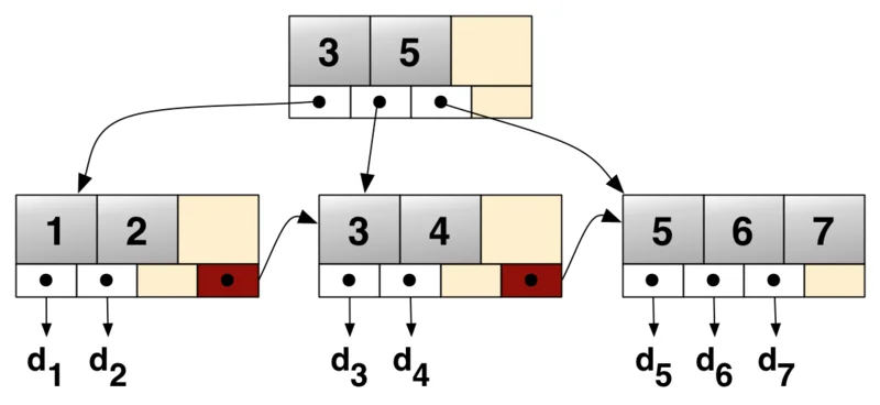
The leaf nodes of a B+ tree contains the data records. The other nodes in the tree are internal nodes and contain a variable (bounded by the branching factor) number of children nodes. The internal nodes only contain key values and are also sorted by key. They point to some pre-defined range in the key-space. Also, the leaf nodes are linked to one another to allow fast range scans.

To analyze the performance characteristics, particularly amplification effects, we establish the following parameters:

• $N$ represents the total number of records stored in the database. Assume records are of approximately constant $O(1)$ size.
• $B$ denotes the capacity of a leaf node block (page) in terms of the number of records it can store. Since we assume records are $\approx O(1)$ in size, each page stores $O(B)$ records.
• $D$ represents the branching factor of the internal nodes, signifying the maximum number of child pointers an internal node can contain (including leaf nodes).

Read Amplification

If the entire B+Tree would fit in memory, a B+Tree would indeed be great. However, in large data use-cases like in InnoDB, the minimum unit of interaction with the storage layer is a database page. A page in a database may be around 4kb or higher (configurable) and contains multiple row entries. The same is true for all indexes. This means, that to read a single row, you need to read the entire page into memory. And similarly, to write a single row, you need to write the entire page back to disk. In the worst case scenario, let’s say a single row is 4KB and your page size is 128KB, and every row read belongs to an unique page, your read amplification is $32 \times$. Not ideal.

Let’s assume that the block size is $O(B)$ & that the branching factor of each node is $O(D)$. That is, each node contain $O(D)$ children (including the leaf nodes). Let’s also assume that the size of all records and pointers etc. are constant. Then the total number of nodes my tree needs to maintain $O(N)$ records is $O(\frac{N}{B})$. Given a branching factor of $D$, the depth of my tree is $O(log_D(\frac{N}{B}))$. A point lookup on a B+ Tree requires traversing the tree from the root down to a leaf page. Since the height of the tree is approximately $O(log_D(\frac{N}{B}))$ a single query requires reading one page at each level of the tree. This gives a read amplification of $O(log_D(\frac{N}{B}))$ disk pages. For range scans, once the starting leaf page is located, the subsequent pages can be read sequentially using the sibling pointers, which is efficient.

Write Amplification

For every write of a record, we would need to write the entire page to memory. Which means, the write amplification is $O(B)$ (records are constant size). However, also note that technically, if we insert into a node that’s already full, we’d trigger a split operation. This split operation in the node can further cascade up the height of the tree triggering more splits. Given that the height of the tree is $O(log_D(\frac{N}{B}))$, in the worst case, we’d trigger $O(log_D(\frac{N}{B}) \times B)$ writes. However, for a B+ tree, amortized over $O(N)$ insertions, the number of splits per insertion is $O(1)$, so this doesn’t matter as much. (Remember that the number of nodes in the tree is $O(N)$ for $O(N)$ insertions, which implies an amortized cost of $O(1)$ splits per insertion.

Space Amplification

The tree (after $N$ insertions) contains $O(\frac{N}{B})$ nodes (pages), which has a memory footprint of $\approx O(N)$. However, the constant factor is likely a significant bit higher than 1. To avoid costly page splits on every insert, pages are often left partially empty. I can’t recall / find the source for this claim, but I remember that on average, B+ Tree pages are about 67% to 75% full… If my memory serves correctly :)

LSM Tree

We’re going to make some assumptions here to simplify the analysis, especially since the deferred nature of writes requires us to do amortized analysis to understand the amplification factors. We’re modeling leveled compaction here. We assume each level to have exactly 1 ‘run’. The new assumptions we make for simplifying analysis are as follows:

1. When does compaction occur? When the size of a level $L_i$ reaches some defined constant limiting size $S_i$.
2. How is $S_i$ modeled? We define a constant ‘scaling / fanout factor’ $k$ and define $S_0 = c$ (where $c$ is some constant) and then define the relationship between the levels as $S_{i+1} = S_i \cdot k$. So for example, if the number of records we allow in $L_0$ is $6$, and we define $k = 2$, then $L_1$ would fit $12$ records, $L_2$ would fit 24, $L_3$ 48, and so on.

Read Amplification

A point query, in the worst-case scenario (the key doesn’t exist), must check every level of the tree. The search path is:

1. Check the active in-memory mem-table.
2. Check Level 0 on disk. Since Level 0 SSTs can have overlapping key ranges, we may have to check every SST file in this level.
3. For every subsequent level ($L_1, L_2, \dots, L_{max}$), we find the single SST that could contain the key and check it.

This means a single logical read can turn into many physical disk reads, making the worst-case read amplification proportional to the number of levels. To mitigate this, most LSM implementations use Bloom Filters. A Bloom filter is a probabilistic data structure that can quickly tell you if a key might be in an SST file, or if it is definitely not. By checking the Bloom filter for an SST (which is small and kept in memory), we can avoid most of the expensive disk reads for keys that don’t exist in that file.

Let’s get into a little more detail here. Remember our assumptions: We’re using a leveled compaction strategy with a fanout factor $k$, where each level $L_{i+1}$ can hold roughly $k$ times more data than $L_i$​. The number of levels is approximately $O(\log_k (N / c))$, where $c$ is the mem-table size limit and $N$ is the total number of records. For point queries:

1. You have to check the mem-table first. This is fast and in-memory: $O(\log(c))$ if it’s implemented as a skip-list or BST. You could probably implement it as a hash table and get $O(1)$ as well. But regardless, it’s some constant time operation and not very relevant so the exact DS implementing it doesn’t matter much.

2. You then need to scan all the SSTs in level-0. This is again, some fixed value. All the SSTs in $L_0$ are pretty small in size and very likely to be in cache since they are the most likely to be read / written from (hot data). Note that most SST scans would be skipped thanks the the bloom filter. And the ones that are scanned are done in $\approx$ constant time. We can more or less consider this set of scans $O(c)$ as well.

3. For higher levels, we need to identify the right SST. This is done by binary searching on the level’s metadata information (which contains information about the start and end keys of each SST in that level). The time complexity of this is $\approx O(\log_k(\frac{N}{c}))$ (There’s $\frac{N}{c}$ records, so we’d have those many levels).

   a. For the highest level $L_{max}$, the data size is $\approx O(N)$. So binary searching on the metadata here is $\approx O(\log(\frac{N}{c}))$. b. For the previous level $L_{max-1}$, the data size is $\approx O(\frac{N}{k})$. So binary searching here is now $\approx O(\log(\frac{N}{kc}))$ c. And so on…

   Summing this up, we get the total number of disk reads required as: $O(\log(\frac{N}{c})) + O(\log(\frac{N}{kc})) + O(\log(\frac{N}{kc^2})) + \cdots + O(\log(\frac{N}{k^nc})) = O(\frac{\frac{\log^2N}{c}}{\log k})$

   But a couple of things come handy here. One, you can store metadata and do all your binary searching on the metadata instead of opening each SST. This makes the binary searches essentially constant time at the cost of some additional (constant) space / extra-work during writes. Further, you’d assume scanning each SST is a disk read, but the bloom filters come in very handy here. Since they help determine (with high probability) if a key is present or not in an SST, they reduce a lot of unnecessary SST opens. Also, since hotter (more recent) data is in upper levels or the mem-table, caching helps a lot. So you could roughly say it’s only $\approx O(\log_k(\frac{N}{c}))$.

For range scans, you may need to merge results from iterators across all levels. Think about it this way, you identify the range $[ST, EN]$ in each level that may contain the keys belonging to the result set (all of $L_0$). However, since we have MVCC, we can have multiple versions of keys, and we could have a situation where $ST \lt a \lt b \lt EN$ but $a \in L_i$ and $b \in L_{j \gt i}$. So we have to somehow read across all levels and merge results together. One common solution is to have essentially a “merge operator.” You have an iterator at the first element greater-than or equal to $ST$ in each range (and less than equal to $EN$). You put the elements each iterator points to in a “merge” priority-queue (with timestamp). The smallest element is popped and streamed to the result set. The iterator that was pointing to this element moves forward and we repeat until each iterator has crossed $EN$. This doesn’t really change the complexity much. For $R$ records, you can expect $O(R \cdot \log_k(\frac{N}{c}))$ complexity (the priority queue would be of size = number of levels).

Write Amplification

The complexity for a single write is constant. $O(1)$ to add to the WAL and time-complexity of chosen DS for the mem-table. In any case, it’s constant. However, most of the write amplification related to LSM trees come during the compaction phase. To model amplification here, we need to try to understand how many disk writes a single write(k, v) operation triggers over the life span of the record $k$. Initially, a single disk-write happens when the mem-table is flushed as a SSTable to disk. After that, every time it’s compacted, we have a disk write. Lets think about what happens during compaction from $L_i$ to $L_{i+1}$:

1. Select the SST from $L_i$ for compaction. Let’s assume the size is $S_i$ records.
2. Identify overlapping key ranges in $L_{i+1}$.
3. Read all records from the selected $L_i$ SST and the overlapping $L_{i+1}$​ SSTs into memory (SSTs are immutable).
4. Merge them: Sort, resolve duplicates (keep the latest version for MVCC), drop tombstones if they cover older data.
5. Write the merged result as new SSTs back to $L_{i+1}$.
6. Delete the old SSTs from both levels.

The bytes written can’t really be made sense of on a per-key basis. However, during this compaction, you can say that the initial $S_i$ records contributed to a write of size $S_i$ + the records in the SSTables in level $L_{i+1}$ that it was merged with. You can compute amplification here for all of those $S_i$ records as $\frac{\text{total records written}}{S_i}$. Let’s see how to compute this better.

Note that all levels span the same key space. However, because $L_{i+1}$ holds $k$ times more data than $L_i$, the data density (number of records per unit of key space) is $k$ times higher in $L_{i+1}$. Let’s assume the size of the key space is $P$. If we compute the data densities for $L_i$ and $L_{i+1}$:

1. $L_i$: The density is $\frac{S_i}{P}$.
2. $L_{i+1}$: Compared so $L_i$, the number of records in this level is now $\approx S_i \cdot k$. So the density is $\frac{S_i \cdot k}{P}$.

Let’s assume keys are uniformly random for the sake of analysis. When we select $S_i$ records from $L_i$ for compaction, these records span some key space $P' \subset P$. The width of this $P'$ depends on the spread of keys, but for the uniformly random case, we can expect the number of records in $L_i$ over $P'$ is $S_i$. So in $L_{i+1}$, because the density is $k$ times that of $L_i$, we can assume that the same range $P'$ will contain $\approx k \cdot S_i$ records.

So, if we look at the original calculation:

This happens at each level a record passes through. A record starts at $L_0$, gets compacted to $L_1$ (rewritten with amplification $\approx k$), then later when that part of $L_1$ compacts to $L_2$ (rewritten again with amplification $\approx k$), and so on, down $\log_k (\frac{N}{c}))$ levels. This gives us a total write amplification $\approx k \cdot \log_k (\frac{N}{c})$. Note that this is average case since we assume uniformly random key distributions. However, in practice, the fact that compaction happens “async” and SSTable’s being immutable and compressible gives huge write amplification wins in comparison to a B+ tree. Merges can be done in parallel and in the “background”, making them much faster for writes.

Space Amplification

Space amplification in an LSM Tree comes from data that is no longer “live” but has not yet been garbage collected by compaction. This includes old versions of updated rows and tombstone markers for deleted rows. Also note that each SSTable in a level in a LSM is responsible for some continuous key range. During compaction, we ensure that only one version of the key (the latest or a tombstone) is preserved. This means that in the worst case, we can have a single key have stale versions copied over once per level. So worst case, we can expect the write amplification to be $O(\log_k(\frac{N}{c}))$. However, in this benchmark by Mark Callaghan on MyRocks (a MySQL engine based on RocksDB which is based on LSM trees) vs InnoDB (the default MySQL engine):

While an LSM can waste space from old versions of rows, with leveled compaction the overhead is ~10% of the database size compared to between 33% and 50% for a fragmented B-Tree and I have confirmed such fragmentation in production. MyRocks also uses less space for per-row metadata than InnoDB. Finally, InnoDB disk pages have a fixed size and more space is lost from rounding up the compressed page output (maybe 5KB) to the fixed page size (maybe 8KB).

Immutability

I figured this is worth spending a H2 heading on :) Most media marketing praises LSM’s for the very fast write speeds and efficient usage of disk. But one very important feature that’s not appreciated enough is their immutability. To be fair, I didn’t really give it much thought either until I met Sunny Bains during a PingCap event in Bangalore and he brought this up. All the fast writes and amplification stuff is good, but one of the best selling points of LSM was the design decision to make SSTable’s immutable. This has a bunch of very profound benefits:

1. Simplicity: That simple decision allows many things to become extremely simple. For example, concurrency is very simple of implement on top of SSTs since they’re immutable. There’s no locks to grab or any other kind of contention to deal with. Concurrent accesses are super simple to implement (in comparison to the shared + exclusive lock complications of a B+ tree). This parallelization allowed Meta (then Facebook) to do significant optimizations on the compaction stage and is one of the key reasons why LSM’s perform so well against B+ trees today.

2. Crash Safety: This also means that things like crashes are easy to recover from. A single WAL is enough to ensure durability. If a system crashes mid-compaction, it doesn’t matter since the original SSTable’s are still intact and valid. We can always resume from a WAL instead of doing pointer shenanigans or maintaining more complicated logs since a crash during a split operation or lock release / grab propagating up the tree is more difficult to model.

3. Efficient Compression + BR: Immutable files are easy to compress / cache. The contents never change, so you don’t need any complex cache invalidation logic. Every SSTable (not in cache) is heavily compressed when stored on disk. Only the SSTable’s which move to memory are uncompressed. This has significant space savings and also means disk space can be used better (<- this is huge). Further, implementing backup restore type operations is super easy since you can just copy the current set of live SSTable’s as is to s3 or something and you’re mostly good for the backup. You don’t need to pause writes (You can pause compactions for a short while instead).

In short, immutability makes so many things awesome and simple and they all convert to pretty important wins for the LSM eventually.