Master’s Theorem

Solving recurrence relations can prove to be a difficult task, especially when there are many terms and factors involved. The master’s theorem is a very useful tool to know about, especially when trying to prove operation bounds for divide and conquer type algorithms. Most such algorithms have some constant factor by which they divide the initial input a certain number of times and recursively perform some operation.

In general, the master’s theorem states that:

A visual depiction of the proof

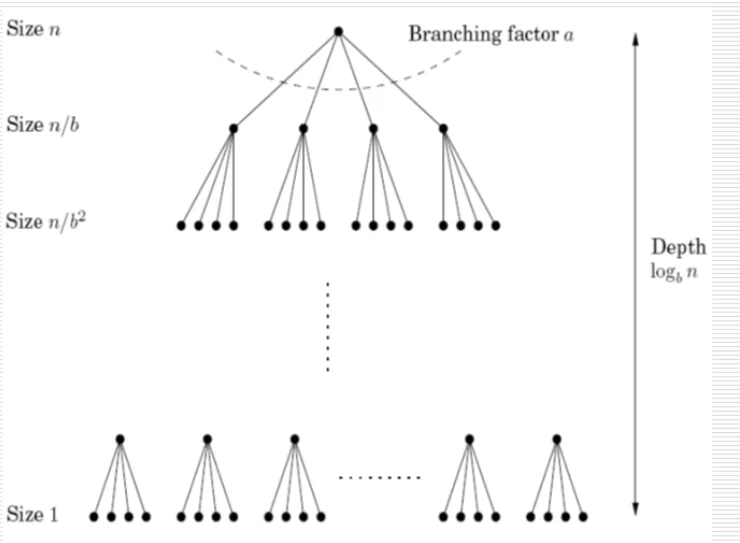
Proof of Master’s Theorem

We can see that the size is divided by $b$ on every level. Therefore, for the size $n$ to go to 1, it will require $log_{b} n$ times. Therefore, the depth of the tree is $log_{b} n$. Also, the number of nodes at level $k$ is $a^k$, therefore the number of leaf nodes is $a^{log_{b} n} = n ^{log_{b}a}$

At the root level, you have 1 node. This node needs to do the following recursive operations.

$T(n) = O(n^d) \ + \ aT(n/b)$ The number of operations the algorithm performs is essentially defined for some input n by this quantity $T(n)$. We notice that for the Master’s theorem, my function is recursively defined. The $O(n^d)$ term is the number of operations I’m doing at the node my recursive algorithm is on. So if I visualize this as a tree, it will have $log_ba$ depth because I’ll have those many divisions of my original input n.

If I had 1 node at the root, at the 2nd level it will split into $a$ nodes on the next level. At the next “level” of my recursion tree, each of these $a$ nodes will split into another set of $a$ nodes. So the depth at the $k^{th}$ level is $a^k$. So at the $k^{th}$ level, I’ll have work equal to the work accumulated by each of my $a^k$ nodes. $a^k$ nodes do $O(n^{'k})$ work. But this is the size of $n^{'}$ at the $k^{th}$ level. The input size $n^{'}$ at the $k^{th}$ level is $\frac{n}{b^k}$ in terms of the original input $n$. (n has been divided by b at each level) So the accumulation of work done at the $k^{th}$ level is essentially

Now if we take the sum of this quantity over all $log_bn$ levels, we notice that this is just a geometric series with first term $a = O(n^d)$ and ratio $r = \frac{a}{b^d}$

Calculating the geometric series will give us the following three results for three different cases of our ratio $\frac{a}{b^d}$.

Cases:

1. $\frac{a}{b^d} \lt 1 \implies a\lt b^d \implies log_ba \lt d$

   The series is decreasing and the dominant term is our first term. This gives us the result, $T(n) = O(n^d)$

2. $\frac{a}{b^d}=1 \implies a = b^d \implies log_ba=d$

   In this case, there are exactly $O(log_bn)$ terms in the series (depth of the tree) and each term is equal to $O(n^d)$. This gives us a simple summation,

   $T(n) = O(n^dlog_bn)$

3. $\frac{a}{b^d} \gt 1 \implies a \gt b^d \implies log_ba \gt d$

   The series is increasing and the dominant term will be the last term of the series.

   $$ n^d(\frac{a}{b^d})^{log_bn} = n^d(\frac{a^{log_bn}}{(b^{log_bn})^d}) = n^d(\frac{a^{log_bn}}{n^d}) \\ a^{log_bn} = a^{log_ba.log_an} = (a^{log_an})^{log_ba} = n^{log_ba} $$

   This gives us the result,

   $T(n) = O(n^{log_ba})$

Matrix Multiplication

Naïve Algorithm: $O(n^3)$

Strassen’s: $O(n^{log_{2}7})$

We imagine the two matrices we have to multiply as consisting of 4 $\frac{n}{2}$ matrices in each matrix.

Notice that this multiplication ends up with us having to calculate the product of 8 such submatrices and the addition of 4. It is evident that multiplication is the bottleneck here. For such an algorithm, we have $T(n) = 8T(n/2) + O(n^2)$ which makes the time complexity $O(n^3)$ as per Master’s theorem. (As $log_ba \gt d$)

However, using a method similar to the same technique used by the Karatsuba multiplication algorithm (Analyzing Fibonacci & Karatsuba Multiplication), we can bring down the number of products to just 7.

Note: This observation is not trivial and does not have a simple construction. But for the sake of documentation, it is shown below.

Strassen’s Matrix Multiplication

The algorithm is as follows. Given

Compute the following terms,

Notice that to compute each of these 7 terms, we only need 7 multiplication operations in total. Now, once computed, we can write the expression $XY$ as follows:

Again as mentioned above, this construction is not intuitive or easy to come up with. With some working out on pen and paper it can be seen that the above construction does indeed yield us the correct result. While it is more complicated, notice that we now only have to perform 7 multiplication operations. The work done at each node is the $n^2$ additions. This lets us write, $T(n) = 7T(n/2)+O(n^2)$. Applying Master’s theorem to this result, we find $log_ba \gt d$ which implies that the time complexity of Strassen’s Matrix multiplication is $O(n^{log_ba}) = O(n^{2.81})$

Finding Median in $O(n)$

The problem of Median finding is as follows. It simply asks, given a list of numbers $S$, find the $\lfloor\frac{n}{2}\rfloor^{th}$ smallest element in the list. In fact, we can generalize this problem to asking, “Given a list of numbers $S$, find the $k^{th}$ smallest element in the list.”

The naïve solution to this problem is simply sorting the list and then just picking the $k^{th}$ smallest element. The correctness of this approach is fairly easy to prove. In a sorted list the condition $a_ican we do better?

Let’s try to apply the same concepts of divide and conquer that netted us promising results in our previous endeavors. Notice that for this particular problem, since our list is unordered, there is nothing to gain by simply splitting the list into $\frac{n}{2}$ halves and solving recursively. The notion of “$k$” does not exist in these halves as we do not have any information about them. Instead, let us consider the division that happens when we pick some arbitrary element $a\in S$.

More formally, if we have some unordered list S, and we pick some element $a \in S$, we can divide the set $S$ into three parts.

Once such a decision is made, we can recursively call our $k^{th}$ order statistic finding algorithm as follows. Let’s call our algorithm selection(S, k) where $S$ is the input list and $k$ is the $k^{th}$ order statistic we wish to find. Then,

$selection(S, k) = \begin{cases} selection(S_L, k) & \text{if} \ k \leq |S_L| \\ a & \text{if} \ |S_L| \lt k \leq |S_L|+|S_a| \\ selection(S_R, k-|S_L|-|S_a|) & \text{if} \ k \gt |S_L|+|S_a| \end{cases}$

Let’s try to parse this recursion.

1. If $k$ is smaller than or equal to $|S_L|$, it means that our “pivot” $a$, was pictorially too far to the right in the sorted list $S$. This essentially means that we overshot our guess for the $k^{th}$ order statistic. Hence we discard every element to the right (pictorially) and recurse on the left part of the list.
2. If $|S_L|$ is lesser than $k$ and $k$ is smaller than or equal to the ranges encompassed by $S_L$ and $S_a$, then it must be true that our $k^{th}$ order statistic is our pivot. Visually, $k$ lies in the range of elements equal to our pivot in the sorted list.
3. If $k$ is greater than the range described in #2, then we undershot our guess for the $k^{th}$ order statistic. This implies that we can discard the left portion of the list and recurse on the right portion. However, we will need to adjust the value of $k$ which is input to it as required.

Notice that in the recursion, we have no guarantee about the size of $S_L$ or $S_R$. The approach of divide and conquer has allowed us to shrink the number of elements we’re worrying about at some step $i$ from $S$ to $max\{|S_L|, |S_R|\}$. However, we have no guarantee about their size.

If we analyze the worst case of this algorithm, notice that the worst case occurs when we pick our pivot in sorted order. In this case, the complexity looks something like $T(n) = T(n-1) + O(n)$. This gives us $T(n) = O(n)+O(n-1)+\dots+O(2)+O(1)$, which essentially gives us a $O(n^2)$ algorithm which is worse than the sort and pick approach.

However, if we analyze the “best” case for this algorithm, notice that if we pick the median as the pivot at each step, we can divide $|S_L|=|S_R|=\frac{n}{2}$. This gives us $T(n) = T(\frac{n}{2}) + O(n)$. Evaluating this, we get $T(n) = O(n)+O(\frac{n}{2})+\dots+O(1)$. This would give us a time complexity of $O(2n) = O(n)$. So in our best case, our algorithm outperforms the sort and pick approach.

Notice the similarity between this algorithm and quicksort. Both have a great best-case time complexity and a very poor worst-case time complexity. They are also very similar in the fact that both their running times are severely affected by the choice of the pivot.

This should clue us into the fact that perhaps trying a randomized approach would give us a desirable result. And we will soon see that a randomized approach does indeed give us a linear expected time complexity. However, it is also possible to provide a deterministic approach that can yield us the linear time complexity we desire. This approach is called the Median of medians and we shall discuss this below. Moreover, notice that since this algorithm is linear, it can be used as a subroutine in the quicksort algorithm to deterministically pick the median as the pivot. This would give us a theoretically very fast quick sort as it can be proved to execute in $O(nlogn)$ for any input. However, practically speaking, the constant factor incurred from running the linear median finding algorithm for every step in quicksort makes it slower in real-time execution. This makes it more preferable to use the randomized quicksort. However, it is pretty cool to note that we can prove quicksort to have an upper bound of just $O(nlogn)$.

Now, coming back to the original problem. If we can pick the median as our pivot, we would get good running time. However, this problem seems counter-intuitive. Our algorithm essentially needs the answer to perform its computation. This isn’t possible. But perhaps it’s possible to put some bound on the size of $S_L$ and $S_R$. Notice that, if at every step of the division, we can guarantee $max\{|S_L|, |S_R|\}$ to be some ratio of $|S|$, we can guarantee linear running time of our algorithm. Evaluating $T(n) = T(\frac{n}{r})+O(n)$, we get

This observation has simplified our problem a little and paved the path for the success of the “Median-of-Medians” approach.

Median-of-Medians

The idea behind the algorithm is as follows. Given some input list $S$ with $n$ elements, perform the following operations recursively.

1. Divide the n elements into groups of 5
2. Find the median of each of the $\frac{n}{5}$ groups
3. Find the median $x$ of the $\frac{n}{5}$ medians

Notice that the time complexity of this is pretty similar to the “linear” running time proof of finding $k^{th}$ order statistics when we are able to divide the input into some ratio at every step. We get $T(n) = 5T(\frac{n}{5})+O(1)$ . Here we consider median finding among 5 elements, a constant time operation. We can solve this recurrence using the Master’s theorem. Notice that $log_ba>d$ which implies the time complexity is $O(n^{log_ba}) = O(n)$.

This means that we now have a linear time algorithm, which can obtain the Median of Medians for some input $n$. Now the question is, how does this help us split $S_L$ and $S_R$ in such a way that we can bound them to some ratio of the original input $n$?

They say a picture is worth a thousand words, and I think you will find the below image quite insightful for the explanation of this proof.

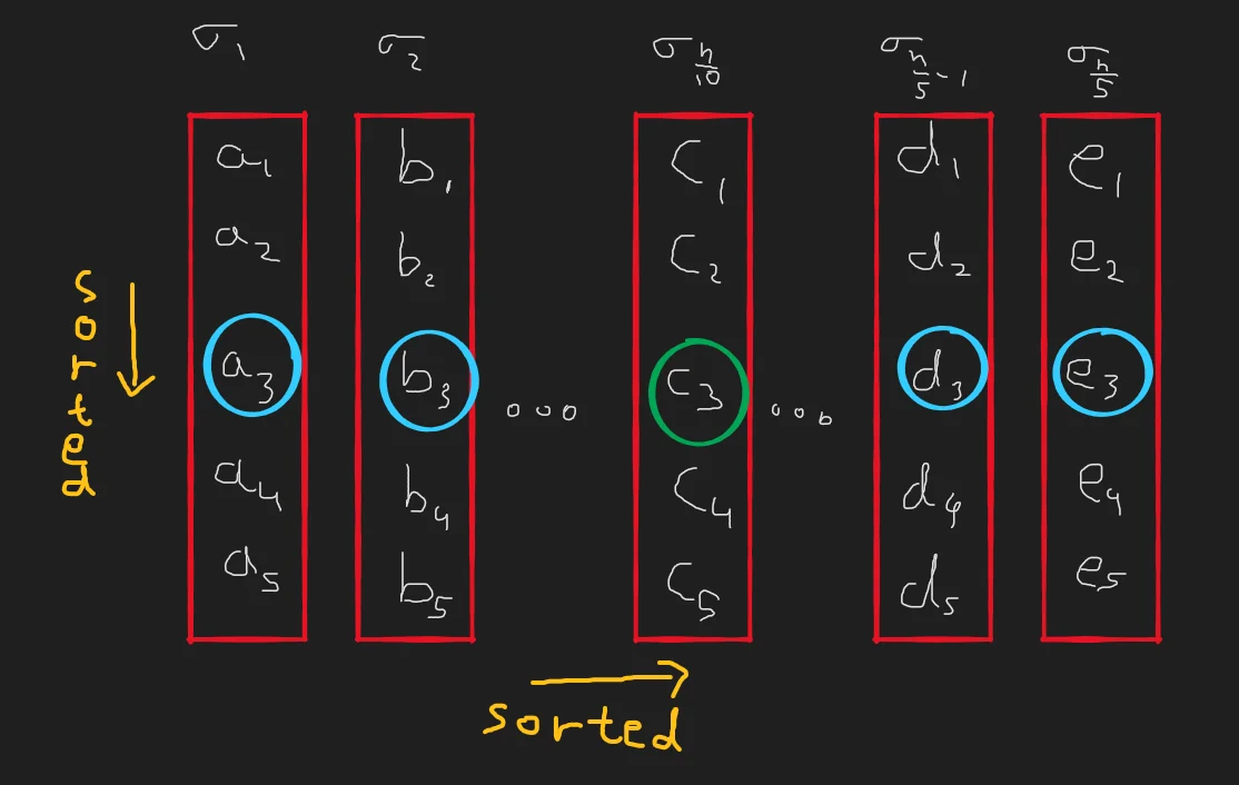
1. Let us divide our set $S$ into $\frac{n}{5}$ lists of 5 elements each and call them $\sigma_1, \sigma_2, \dots, \sigma_{\frac{n}{5}}$.
2. For visualization’s sake, let us picture each of these lists in sorted order vertically. For example, in $\sigma_1$, $a_1\leq a_2 \leq a_3 \leq a_4 \leq a_5$ holds. Notice that this implies that in every list, the third element must be the median.
3. Now, let us sort the lists themselves horizontally by their median value. That is, in the picture below, $a_3\leq b_3 \leq c_3 \leq d_3 \leq e_3$ is true. Notice that this implies that in the below picture, the 3rd element in list $\sigma_{\frac{n}{10}}$is the median-of-medians.

Now that our elements are now ordered both vertically and horizontally, let us try to place bounds on the division that picking the median of medians grants us.

Notice that in the above picture, because $c_3$ is the median of medians, it must be greater than $a_3$ and $b_3$. More formally, $x_3\in \sigma_{\frac{n}{10}} \geq x_3\in \sigma_{i<\frac{n}{10}}$. Further, because $x_3\in\sigma_i$ is greater than or equal to all $x_1, x_2 \in \sigma_i$, our median-of-medians is greater than or equal to every $x_{i\leq3}\in\sigma_{i\leq\frac{n}{10}}$. Or to put it more simply, it must be greater than equal to everything on this picture that is painted in pink.

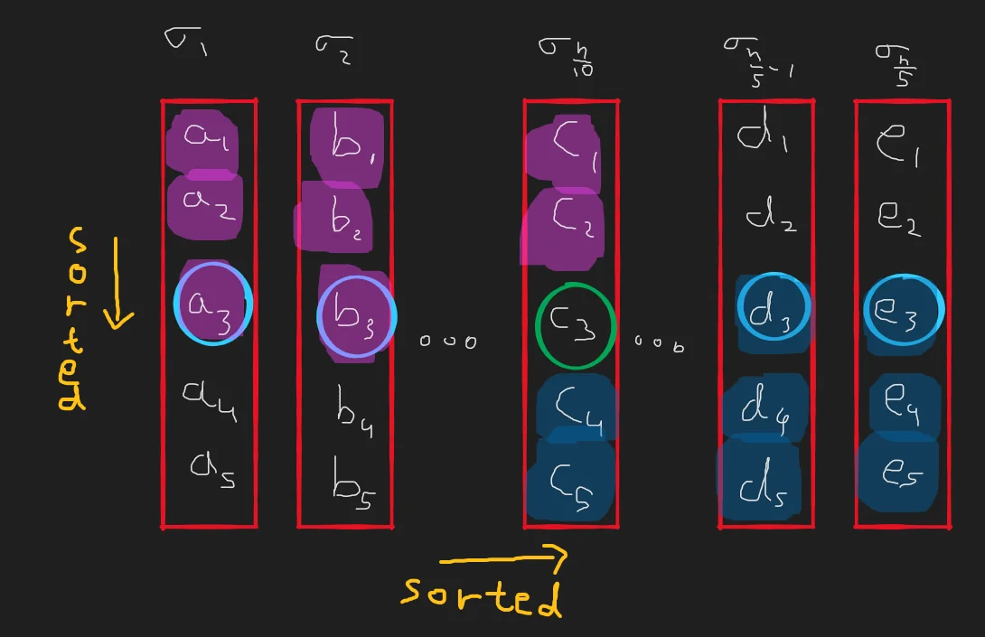
A similar statement can be made about everything it is lesser than or equal to. Everything painted blue in the above diagram must be greater than or equal to our median-of-medians.

If that makes sense, let’s try to formalize and state our argument more quantitatively now. Once we have chosen our pivot as the median-of-medians, the set of all elements lesser than equal to the pivot is essentially just $S_L$. So… how do we enumerate $|S_L|$ or $|S_R|$?

Notice that there are $\lceil \frac{n}{5} \rceil$ lists in total. Out of these, we can enumerate one-half of the lists (including the list containing the median-of-medians) as $M = \lceil \frac{1}{2} \lceil \frac{n}{5} \rceil \rceil$. Each of these $M$ lists contains 3 elements that are lesser than equal to the pivot. This gives us $|S_L| \geq 3M.$ We can obviously remove the pivot itself while recursing and this would give us $|S_L| \geq 3M-1$. Similarly, for $|S_R|$, we might have to remove the last set if $n$ was not perfectly divisible by 5. This would give us the same bound $\pm c$. Since $c$ is pretty small we’ll just choose to ignore it in our calculations.

This gives us

Conclusion

We came up with an algorithm to find the median-of-medians in linear time. And we have managed to prove that picking the median-of-medians as the pivot, lets us divide the original set into $S_L$ and $S_R$ such that their size is always bound to be greater than some ratio of the input n. These 2 facts combined give us the linear time $k^{th}$ order statistics finding algorithm.

To state this more formally,

• We can find the median of medians for some input $n$ in linear time.
• Using the median-of-medians as pivot, we guarantee a division of $S$ into sets such that the next step of our $selection(S, k)$ algorithm will receive as input $S'$ which can be expressed as a ratio of the input $n$. $|S'| \leq \frac{7}{10}n$
• This implies that the total runtime of our algorithm is linear

References

These notes are old and I did not rigorously horde references back then. If some part of this content is your’s or you know where it’s from then do reach out to me and I’ll update it.

1. Professor Kannan Srinathan’s course on Algorithm Analysis & Design in IIIT-H