Greedy Algorithms

Picking off from Activity Selection & Huffman Encoding, the Greedy idea is as follows. At every step, our algorithm picks the locally optimum choice in the hope that this choice will also be the global optimum. The greedy idea is often the easiest to come up with. Picking the local optimum, in some sense, is often a much easier problem to solve than picking the global minimum. Picking the global minimum often requires seeing ahead to figure out if a global optimum can be reached by picking non-locally optimum choices.

This often requires recursively solving and there are techniques to speed up computation, but just looking at the local options and picking the best option is much easier in general. The implementation is simple as well. We only need to consider the local choices.

These properties of greedy algorithms make them quite desirable. An easy to implement an algorithm that is also very fast? That’s a great algorithm. Except, for one caveat. As with any algorithm, the first most important thing to prove about it is its correctness. This is sadly the case with most greedy algorithms, they fail this test. Picking the local optimum is often not the right way to proceed in many algorithms. They might give a desirable result, something close to the global optimum. But not the global optimum itself. And often, it will be possible to generate a counter-case where the greedy solution can be forced to produce a very poor result.

If a shoddy, quick solution that provides a “good” result in most cases is the desired result, then the greedy solution is a great choice! In fact, there are many “hard” problems today whose global optimums cannot be computed in feasible time, even with the best-known algorithms for them. In such situations, the best we can hope is to produce a good greedy solution that generates a “good” result and hopes that it is close to the global optimum.

Matroid Theory

Matroid theory gives the sufficient condition for greedy strategies to be applicable to a problem. If we can express a problem in the terms described by Matroid theory, then we can be guaranteed that a greedy solution exists for this problem. From here on forth, when we say “greedy solutions”, we will refer to greedy solutions that always give the global optimum. Also, note that the reverse is not true. Matroid theory is simply a sufficient condition. If a problem does not fit the matroid theory, it does not mean that it cannot have a greedy solution. Dijkstra is one such problem that does not fit the terms described by Matroid theory, yet has a greedy solution.

The Minimum Spanning Tree (MST) problem

The MST problem asks the following question, “Given some undirected graph G, find a fully connected tree such that it contains every vertex of the graph G and the set of all edges of the tree must be a subset of the edges of G and its total cost is minimized.”

More formally

Given some undirected graph $G = \langle V, E\rangle$ where each edge has some cost $w_e$ associated with it, find a tree $T = \langle V, E'\rangle$ where $E' \subseteq E$ and the total cost of the tree $\sum^{e \in E} w_e$ is minimized.

Consider the naïve approach which involves finding every possible spanning tree of the graph and finally outputting the one with the least cost. This is not feasible as the number of spanning trees we can generate for some graph $G$ grows exponentially.

This is where the idea of “Greedy” comes in. However, to facilitate proving the correctness of our solution later, let us cover an interesting property about graphs first.

The Cut Property

Cut

In graph theory, we define a cut as a partition that divides a connected graph into two disjoint subsets.

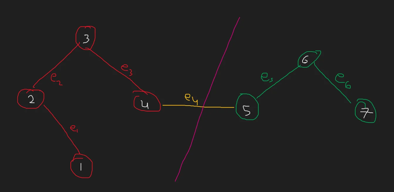
Notice that in the above graph, the “cut” depicted by the pink line divides our graph into two connected disjoint subgraphs. A cut can remove multiple edges, but the end result is two disjoint connected subgraphs.

Here we also define what is known as the Cut Set. It is simply the set of all edges in the cut. That is, it is the set of all edges which must be removed to achieve the result of the cut. In the above example, the cut set would be $E_c= \{e_4\}$

The Cut property - Statement

Let’s say $X$ is the set of all the edges belonging to the MST of some undirected graph $G$.

Now, pick some subset of nodes $S$ such that none of the edges in $X$ provide a connection between 2 vertices in $S$ and $S^c$. In more intuitive terms, this subset must either all belong to the MST or all not. We can now imagine this as a cut between all the nodes in the MST and all the nodes not included in the MST yet.

The cut property states that the minimum weight edge in the cut set should be included in the minimum spanning tree of the graph $G$. That is, the minimum weight edge that crosses $S$ and $S^c$ must be a part of the MST of the graph.

Proof:

• We have some set of edges $X$ which belong to the MST $T$ of our undirected graph $G = \langle V, E \rangle$.
• Let us begin by assuming that we have picked some edge $e$ which is not the minimum weight edge in the cut set
• If we do so, it will lead to constructing a different MST $T'$ of our graph compared to the MST that we would generate if we included the minimum weight edge $e_{min}$.
• Now, because $T'$ is an MST, it must be connected and acyclic. Also, by proof of its construction, $e_{min}$ does not belong to $T'$
• Now, since the graph is a tree, if we include $e_{min}$ to $T'$, notice that there must exist some edge(s) in $e' \in E'$ such that $e_{min}$ forms a cycle with $e'$. [$E'$ is the edge set of $T'$ ]. This must be true as every node is connected, and the graph is acyclic. This implies there is a unique path between any 2 pairs of vertices in the graph. If a new edge is added connecting two nodes, a new path is created between them which creates a cycle.
• Now, by nature of how $T'$ was constructed, $w_{emin} \lt w_{e'}$. If this was not true we would have picked $e'$ to be $e_{min}$
• Next, remove edge $e'$. Notice that removing an edge from a cycle does not make the graph acyclic. Further, we added and subtracted one edge each. This implies that the number of edges in the graph is still $|V|-1$. This implies that the graph must be acyclic as well. That is, our new graph is a tree.
• The cost of our new tree is $W_{T'} - w_{e'} + w_{emin}$ .
• $W_{T'} - w_{e'} + w_{emin} \lt W_{T'}$ as $w_{emin} \lt w_{e'}$. This implies that $T'$ is not the MST as a better tree can be constructed which includes $e_{min}$.

Kruskal’s Algorithm

Kruskal’s approach isolates all of the nodes in the original graph, forming a forest of single node trees, and then progressively merges these trees, merging any two of all the trees with some edge of the original graph at each iteration. All edges are sorted by weight before the algorithm is run (in non-decreasing order). The unification procedure then begins: choose all edges from first to last (in sorted order), and if the endpoints of the presently selected edge belong to separate subtrees, these subtrees are merged, and the edge is added to the answer. After iterating through all of the edges, we’ll find that all of the vertices belong to the same sub-tree, and we’ll have the solution.

Further, note that there may be multiple possible solutions. Kruskal will simply give us one such solution.

Proof

Most greedy algorithms often have their proof in induction, as it is a methodical and elegant way to approach the reasoning of picking the local optimum to get the global optimum. Notice that at every step of the algorithm, we pick the local optimum. That is, we pick the lowest weight edge that belongs to the cut set of the MST and the graph. Hence, by the cut property, the edge we pick must belong to the MST. Doing so repeatedly allows us to pick all $n-1$ edges for the graph.

A small problem

Notice that sorting takes $O(nlogn)$ time. But however, checking if a chosen edge belongs to the cut set or not takes $O(n)$ for each edge. This is not ideal and pushes the algorithm to the time complexity of $O(n^2)$. However, it is possible to eliminate this cost by introducing a data structure that can perform a unification operation and parent lookup operation in an amortized constant time complexity. This will bring down the total time complexity of Kruskal’s to $O(MlogN)$ where $|E| = M, |V| = N$.

Disjoint Set Union

The DSU is a data structure that allows for queries of two types.

1. Merge 2 sets
2. Query the root element of some set $S$

The idea is to maintain a structure that maintains the sets as nodes in a tree where the root is the primary identifier of any set and a merging operation is simply the unification of two trees.

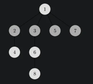
The DSU is initially initialized as an array like so dsu[i]=i. dsu[i] essentially contains the parent element of set $i$. If $dsu[i]=i$, then $i$ is the root node. Following is the code for the DSU:

Querying for parent:

int parent(int i){
    if(dsu[i]==i) return i;
    else return parent(dsu[i]);
}

Looking at just this, it is easy to come up with a case for which this algorithm will take $O(n)$ time. However, by introducing a small factor in the merging step, it is possible to guarantee $O(logn)$ complexity. Here is the code for the unification of two sets in the DSU.

Query to merge two sets:

void unify(int a, int b){
    a = parent(a);
    b = parent(b);
    if(rank[a] < rank[b])
        swap(a, b);
    dsu[b] = a;
    if(a!=b && rank[a] == rank[b])
        rank[a]++;
}

What is rank[x]?

We can think of rank[x] as simply a variable that helps us construct balanced tree structures when we perform the merging operation. Notice that the following statements always hold true for rank[x].

1. For all $x$ in our DSU, $rank[x] \lt rank[parent(x)]$
2. Let’s say some root node in our DSU has rank $k$. This implies that this root node has at least $2^k$ nodes in its subtree. Why? Notice that to make a tree of rank $k$, we need at least two trees of rank $k-1$. if(a!=b && rank[a] == rank[b]) implies this. We can then extend this by induction to prove this.
3. From statement 2, it is implied that if there are $n$ elements in the DSU, at most $\frac{n}{2^k}$ nodes can have rank $k$

This gives us a balanced tree construction in the unification stage that ensures that our $parent(x)$ queries are no more than $log(n)$ per query.

However… can we do better?

It turns out that indeed, we can!

Path compression

Let’s consider the following alternative to our initially proposed parent(x) function.

int parent(int i){
    if(dsu[i]==i) return i;
    else return dsu[i] = parent(dsu[i]);
}

Notice that the only line that has changed is the last line. We simply assign $DSU(i)$ to the parent of $DSU(i)$ at every query operation. This has the effect of shortening the path we must traverse on our journey to find the root node from any child.

Say we break the numbers in intervals of $log^*n$. We get the following split.

Notice the following

1. If a node $x$ on the path to the root is of the same rank as the parent, say in the interval $[k+1, \dots, 2^k]$, then the parent can increase its rank a maximum of $2^k$ times. After these many jumps, it is incremented to the next interval.
2. If a node $x$ on the path to the root has a rank lesser than the rank of the node’s parent, then there can be only $log^*n$ nodes of this type.

This tells us that $2^k\times|\text{nodes with rank} \gt k| \leq nlog^*n$

Combined with the unification via rank optimization, it is possible to prove that the amortized bound over all operations can be as low as $O(\alpha(n))$ where $\alpha(n)$ is the inverse Ackermann function. This can be reasonably approximated to a constant as the inverse Ackermann function is a function that grows extremely slowly. In fact, $\alpha(n) \lt 4$ for $n \lt 10^{600}$.

Code!

Below are links to C++ implementations of both the fully equipped Disjoint Set Union data structure and Kruskal’s. algorithms-notebook/dsu.cpp at main · akcube/algorithms-notebook algorithms-notebook/kruskals.cpp at main · akcube/algorithms-notebook

References

These notes are old and I did not rigorously horde references back then. If some part of this content is your’s or you know where it’s from then do reach out to me and I’ll update it.

1. Professor Kannan Srinathan’s course on Algorithm Analysis & Design in IIIT-H
2. Disjoint Set Union - cp-algorithms