Let’s learn another really cool tool that can be used to solve optimization problems, network flows!

What is the network flow graph?

A network flow graph $G = \langle V, E \rangle$ is nothing but a directed graph, with 2 distinctive features.

1. It has 2 distinct vertices $S$ and $T$ marked. $S$ is the source vertex and $T$ is the sink vertex. These vertices are distinct.
2. Every edge $e \in E$ has some capacity $c_i$ associated with it. It is implicitly assumed that $\forall e \in E, c_i = 0$.

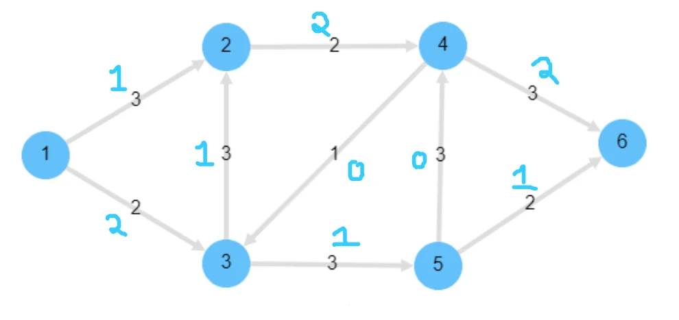
An example of one such graph is given below

Here, $S = 1$ and $T = 6$. We will use this same example when discussing further ideas.

The problem

The problem that network flow attempts to solve is pretty simple. It asks the questions, “Given an infinite amount of “flow” at source $S$, what is the maximum amount of “flow” you can push through the network at any point of time and reach sink $T$?”

An intuitive way to think about this is to pretend that the source $S$ is an infinite source of water and that the capacities on each edge are sort of like the maximum amount of water that can flow through each of the “pipes” or edges. If we think of edges in terms of pipes, the question basically asks how much water we can push through the pipes so that the maximum amount of water reaches sink $T$ per unit time.

Why is this helpful? Think about traffic scheduling, for example, we could replace water with traffic and the problem would be similar to scheduling traffic through a busy set of streets. Replace it with goods flowing in a warehouse system and we begin to see how powerful this model of the optimization problem is.

To define this more formally, the only primary constraints are as follows:

1. The flow through any edge must be $\leq$ the capacity of that edge.
2. The flow entering and leaving any given vertex (except $S$ or $T$) must be the same. (Pretty similar to Kirchhoff’s current laws.)

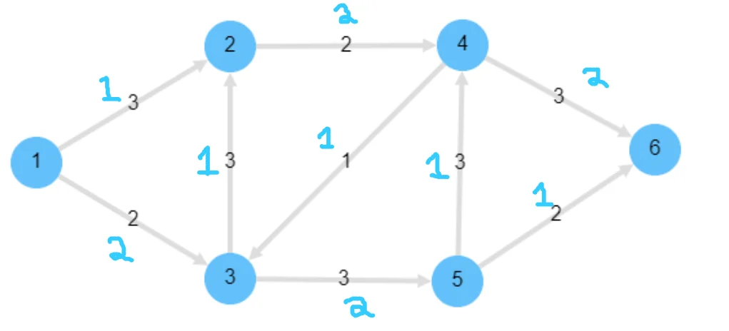
Here is an example of a valid network flow assignment:

We can manually go over every vertex and ensure that the two constraints are obeyed everywhere. Further, notice that the flow of this network $= 3$. (Just sum up the flow going to $T$, i.e., the edges incident on $T$)

An interesting observation is that we appear to have “cyclic flow” within our graph with this particular assignment of flow. Eliminating this does not change the total flow going to $T$, so this is pretty much the same assignment without that cyclic flow within the network:

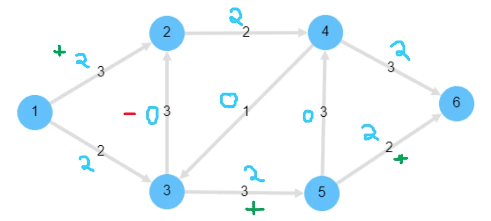
But what about the max flow assignment for this network? is 3 the maximum flow we can achieve? Or can we do better? After a bit of fiddling around, we can notice that we can do better by pushing more flow on the bottom half of this network instead of sending 1 flow up to the top from node 3. Fixing this ends up giving this network:

It can be proven that we cannot do better than this for this particular network. The max flow of this network is 4.

Hopefully, the above examples have managed to convey the true difficulty that flow algorithms face. Solving network flow is not easy, primarily because from any given state, the optimal state might not be reached by just monotonically increasing flow through edges. We might have to reduce the flow through some edges to increase the flow in others. Changing the flow amount through any one edge ends up affecting the entire network. So we need to find ways to iteratively increase the flow in our network, BUT it is not a monotonic increase. So we must sometimes backtrack and reduce flow in some edges. But perhaps by focusing on monotonically increasing the max flow of our network, we might be able to figure out a proper algorithm that incorporates this backtracking. This is the primary goal we keep in mind when trying to solve max flow.

Defining the problem formally

Some useful notation

For the remainder of this article, we will use “implicit summation” notation. All sets will be named by capital letters, and whenever we use sets in the place of elements like for example $f(s, V)$, this means the summation of flow $\sum_{v\in V} f(s, v)$. We use this notation to simplify the math we will be writing.

Formal definition

Flow: We define the flow of a network $G$ as a function $f:V \times V \to R$ satisfying the following 3 constraints,

1. $\forall u,v \in V, f(u, v) \leq c(u,v)$. That is, flow through any edge must be less than the capacity of that edge.
2. $\forall u\in V - \{ s, t \}, f(u, V) \implies \sum_{v\in V}f(u,v) = 0$. That is, flow entering and exiting every node except source and sink is 0. It is conserved.
3. $\forall u, v \in V, f(u,v) = -f(u,v)$. This is not the flow between two vertices, given any two vertices on the network $u$ and $v$, the flow going from one vertex u to v should be the negation of the flow from v to u. This property is called skew-symmetry.

Defining flow

Let us denote the value of the flow through a network by $|f|$. Then we define this quantity as

Intuitively, this is essentially all the flow (sum) that is going from the source node to every other vertex on the graph. It is important to note that the summation is not of all positive terms, if there is flow going from some vertex $v$ to $s$, then this term would be negative (skew symmetry).

Using this, it is possible to prove that $|f| = f(s, V) = f(V, t)$. That is, it is all the flow going to vertex $t$ and is more “intuitive” to understand as the definition of flow. But before we can prove this, let’s go over some key properties of flow-networks which we can derive from the constraints.

Properties:

1. $f(X, X) = 0 , X \subset V$, this is derivable from skew-symmetry.
2. $f(X,Y) = -f(Y,X), X,Y \subset V$. Direct consequence of skew symmetry.
3. $f(X \cup Y, Z) = f(X,Z)+f(Y,Z) \text{ if } X\cup Y = \phi$. If the intersection of $X$ and $Y$is null, then we can safely add the two flows separately as there is no risk of double counting.

Now that we know these properties, let’s prove it!

Let’s start from the definition of our flow amount $|f|$. Using property 3, we can transform it to mean

This is intuitively just saying that flow from $s \to V$ is the negative of the flow from other vertices to all vertices. This is because flow within non-source-sink vertices is 0 and they must all flow out the sink. Now, notice that we want to try to prove that $|f| =f(V,t)$. To do this, we will attempt to isolate $t$ from the above equation using the 3rd property again.

The tricky part here is understanding why $f(V-s-t,V) = 0$. This is because of flow conservation. Flipping it around, we get $f(V, V-s-t)$. By the 2nd constraint imposed on our flow network, this quantity is constrained to be 0 always. Hence we have now proved that

Ford-Fulkerson

Residual networks

We denote the residual network of a flow network $G$ by $G_R(V_R, E_R)$.

The only constraints on the edges are that all the edges have strictly positive residual capacities. 0 means the edge is deleted. And, if $(u,v) \notin E, c(v,u) = 0, f(v,u) = -f(v, u)$

Essentially, $\forall e\in E_r, c_{Re} = c_e-f_e$. The residual edges represent edges that “could” admit more flow if required. Here $c_e$ is the capacity of the edge in the original flow graph and $f_e$ is the flow passing through the edge in the original flow network.

The idea behind these edges becomes more apparent when we actually construct the network.

Consider the old suboptimal max flow network we had.

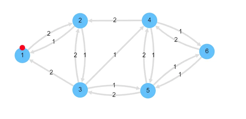
We’ll begin by constructing the residual graph for this network. Remember, for each edge in the network, we add an edge with capacity $c_e - f_e$ as long as this quantity is $\gt 0$. And now, to respect the last constraint, we must ensure that we add a back-edge in the opposite direction with value = $f_e$ as long $f_e \gt 0$. This is the key idea behind what the residual network hopes to accomplish. Recall back when said one of the reasons the flow problem was very difficult was because it is very difficult to account for having to reduce flow in some edges to increase max flow? This residual network is what helps the algorithm get around this problem. Here is the residual network:

Now, the Ford Fulkerson algorithm becomes extremely simple. It simply says, use any graph traversal algorithm such as BFS or DFS to find an augmenting path in this graph, and apply it to the original graph.

We formally define an augmenting path as a path from $s_R$ to $t_R$ in the residual graph. Recall that every edge in the residual graph must be a positive value. If such a path is found, then it must be possible to increment the value of max flow in the network by at least 1. This is because the residual graph is essentially an entire encoding of every possible increase/decrease in flow that we can perform on the original graph. The presence of a path with all edges $\gt 0$ implies I can increase flow from $s_R$ to $t_R$ by at least 1.

If this is understood, the Ford Fulkerson algorithm becomes pretty simple.

Pseudocode

1. Construct the residual graph for some given flow network $G$
2. While we can find an augmenting path in the residual graph:
   1. Get the min of the edges that constitute this path and increment the flow in the original graph by this value along the edges in the residual graph. If it is a direct edge, increment by min. If it is a back-edge, decrease flow by min.
   2. Reconstruct residual graph.
   3. Repeat. If no more augmenting paths are found, we have achieved max flow.

Proof

Why does this algorithm work optimally all the time? To prove the correctness of this algorithm, we will first prove the correctness of the Max-flow, Min-cut theorem.

Max-Flow, Min-Cut

The theorem states that the following statements are equivalent.

1. $|f| = c(S, T)$ for some cut $(S, T)$.
2. $f$ is the maximum flow.
3. $f$ admits no augmenting paths.

We will prove this theorem by proving $1 \implies 2 \implies 3 \implies 1$.

Proving $1 \implies 2$

We know that $|f| \leq c(s, t)$ for any cut $(s, t)$. Hence, if $|f| = c(s, t)$ then $f$ must be the maximum flow through this network.

Proving $2 \implies3$

We can prove this by contradiction. Assume that there existed some augmenting path. Then this would imply that we could increase the max flow by some amount, hence contradicting the fact that $f$ is the maximum flow. Hence $f$ cannot admit any augmenting paths.

Proving $3 \implies 1$

Let us assume that $|f|$ admits no augmenting paths. That means, we have no path from $s$ to $t$ in $G_R$. We now define two sets $S = \{v\in V : \text{ there exists a path in } G_R \text{ from } s \to v\}$. The other set is defined as $T = V-S$. Trivially, $s \in S$ and $t \in T$, as I cannot reach $t$ from $s$. Therefore, these two sets form a cut $(S, T)$.

Now, we pick two vertices $u \in S$ and $v \in T$. Now, by definition, there is a path from $s$ to $u$. But no path from $u \to v$. Otherwise $v \in S$, which is false.

Now, $c_R(u,v)$ must be zero. $c_R(u,v)$ is by definition always positive. Now, if $c_R(u, v) \gt 0$ it would imply that $v \in T$. This is a contradiction. Therefore, $c_R(u,v) = 0$.

Now, we know that $c_R(u, v) = c(u,v) -f(u,v) \implies f(u,v) = c(u,v)$

For our arbitrary choices of $u \in S$ and $v \in T$, we arrive at the conclusion that $f(S, T) = C(S, T)$.

Since $1 \implies 2 \implies 3 \implies 1$, the Min-Cut Max Flow theorem is true.

Proving Ford-Fulkerson

Now, the Ford Fulkerson algorithm terminates when there are no longer any more augmenting paths in $G_R$. According to the Maxflow MinCut theorem, this is equivalent to our network reaching maximum flow. Hence we have proved the correctness of our algorithm.

Complexity

It is easy to see that for integral capacities and flow constraints, finding an augmenting path implies increasing the value of maximum flow by at least one. This means that the algorithm will at least increment flow in network by 1 per iteration. Hence it will terminate and we can bound the complexity to $O((V+E)U)$ where $V+E$ is the complexity of the BFS and $U$ is max flow.

For non-integer capacities, the complexity is unbounded.

This… isn’t great. Because our complexity depends on the maxflow of the graph. If we construct a graph such that at each iteration, we have worst case and the algorithm increases flow in the network by only one unit and the capacity on the edges is large, we might end up doing millions of iterations for a small graph.

Edmond-Karp

Edmond and Karp were the first to put a polynomial bound on this algorithm. They noticed that BFS implementations of Ford Fulkerson’s outperformed DFS versions a lot. Upon analyzing these implementations, they were able to put a polynomial bound on the problem. Their were able to reduce it the following bound: $O(VE^2)$. The coolest part about this is that this is true even for irrational capacities!

The intuition is, that every time we find an augmenting path one of the edges becomes saturated, and the distance from the edge to $s$ will be longer, if it appears later again in an augmenting path. And the length of a simple paths is bounded by $V$.

Dinics

Dinic’s algorithm solves the maximum flow problem in $O(V^2E)$.

More recent research

The asymptotically fastest algorithm found in 2011 runs in $O(VElog_{\frac{E}{VlogV}V})$ time.

And more recently, Orlins algorithm solves the problem in $O(VE)$ for $E \leq O(V^{\frac{16}{15}-\epsilon})$ while KRT (King, Rao and Tarjan)’s does it in $O(VE)$ for $E \gt V^{1+\epsilon}$

There’s a lot of research going on in this field and we know no proven lower bound for this algorithm. Who knows, we might be able to get even faster! Techniques like push-relabel, with a greedy optimization have managed to get a lower bound of $O(V^3)$. This modification was proposed by Cheriyan and Maheshwari in 1989.

References

These notes are old and I did not rigorously horde references back then. If some part of this content is your’s or you know where it’s from then do reach out to me and I’ll update it.

1. Incremental Improvement: Max Flow, Min Cut - MIT OCW 6.046J - Srinivas Devadas