OtterTune - Automatic Database Management System Tuning Through Large-Scale Machine Learning
Interactive Graph
Table of Contents
Abstract
Tuning a MySQL node (well) can be a challenging task for most DBAs, primarily because the variables that control the performance of the node are all inter-dependent on each other. A simple version of this problem might be dealing with the branch predictor in a processor. For strided accesses branch prediction might do a great job, but it might be counterproductive in a workload that has completely random accesses as it will fetch several useless lines into cache causing some thrashing. Add dependent variables like fixing a good “cache size” for a workload and we’re immediately forced to try every combination of values to pick the “optimal” values for a workload since we cannot solve them independently.
In one of his talks, Andy mentions how whenever a developer working on MySQL / Postgres implements something new where they have to decide on a “good” size for a buffer or similar, they just expose it as a variable that can be configured. This is a problem not just restricted to database systems, you’ll find similar themes in any program that has to crunch through a lot of data. For example, genomic pipelines which have to crunch through gigabytes of data using heuristic algorithms (which have extreme random-access patterns) also provide a bunch of variables & caching mechanisms you can tune to improve performance. I believe the automation and ideas described in this paper can be used to tune a lot of things beyond DBMSs.
Abstract Database management system (DBMS) configuration tuning is an essential aspect of any data-intensive application effort. But this is historically a difficult task because DBMSs have hundreds of configuration “knobs” that control everything in the system, such as the amount of memory to use for caches and how often data is written to storage. The problem with these knobs is that they are not standardized (i.e., two DBMSs use a different name for the same knob), not independent (i.e., changing one knob can impact others), and not universal (i.e., what works for one application may be sub-optimal for another). Worse, information about the effects of the knobs typically comes only from (expensive) experience.
To overcome these challenges, we present an automated approach that leverages past experience and collects new information to tune DBMS configurations: we use a combination of supervised and unsupervised machine learning methods to (1) select the most impactful knobs, (2) map unseen database workloads to previous workloads from which we can transfer experience, and (3) recommend knob settings. We implemented our techniques in a new tool called OtterTune and tested it on three DBMSs. Our evaluation shows that OtterTune recommends configurations that are as good as or better than ones generated by existing tools or a human expert.
The Problem
Big Data Era
Processing & analyzing large amounts of data is crucial in the “big data” era we live in now. We measure the performance of these data processing systems in metrics like throughput & latency. Both of these quantities can be significantly impacted by the parameters a DBMS is configured with for a given workload and cluster spec.
Too Much To Tune
Modern database management systems are notorious for having a bazillion parameters that can be “tuned” to better fit the user’s runtime environment and workload.
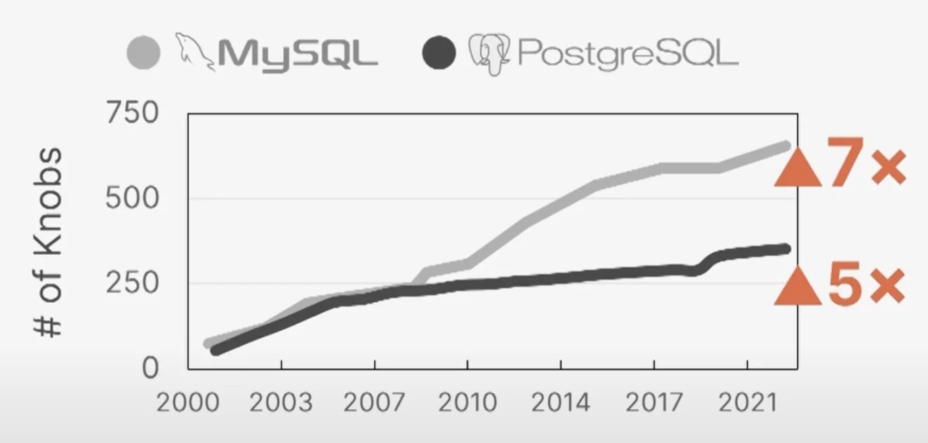
In the past 20 years alone, MySQL has grown from having some 30 knobs or so to 700+ now. That’s simply far too many parameters for any single human or even group of humans to optimize. You might be able to classify some parameters as useless (name of output file, port, etc.) but a lot of other parameters may be inter-related to each other and affect performance significantly. The optimal configuration cannot be reached by distributing and solving independently. And solving it individually is beyond what humans can reason about.
Previous Attempt(s) Shortcomings
The authors claim that most of the previous attempts either suffered from vendor lock-in or they required integrating several manual steps in the process. They were more so configured to “assist” DBAs than automate the tuning process.
All of these tools also examine each DBMS deployment independently and thus are unable to apply knowledge gained from previous tuning efforts. This is inefficient because each tuning effort can take a long time and use a lot of resources.
Expensive Humans, Cheap Machines
This is the classic problem of some designs being optimized for cost-savings in the old days when human labour was cheap and computers were extremely expensive to acquire. Nowadays, especially with the advent of the Cloud, getting access to expensive hardware has become much cheaper. In contrast, the supply of DBAs who are capable of making any decent progress in tuning the complex DBMSs we have today have dwindled, consequently also making them extremely expensive labour for companies.
Tuning Is A Difficult Problem
Dependencies
Standard ML Problem?
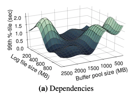
Knobs cannot be tuned independent of each other. A subsets of knobs may end up changing the effect of a different subset. This was the figure they obtained just plotting Log file size vs Buffer pool size. In reality we’re trying to find a global optimum for an $n$-dimensional function (where $n$ is the number of knobs). This alone would be a classic machine learning problem.
Not Really
However, it’s not that simple. For one, this $n$ dimensional function is fixed only for a very specific workload and for a specific system configuration that it runs on. If the workload or configuration changes, the function changes. This makes using “past” data for optimization very difficult. Further, we also cannot afford to run the workload with varying configurations many times since the costs will easily shoot through the roof. The function is also not perfectly constant between multiple replays of the same workload but should be close enough.
Non-Reusability
Continuing the previous section, non-reusability of data is by far the hardest problem here. If we could just use the data we have across hundreds of databases, we can just collect a lot of data and then easily optimize things. But even for a fixed instance & database combination, a change in the workload can drastically change the function we are trying to optimize. This means for each database, instance & workload combination, we have to run an expensive data collection & tuning process.
OtterTune
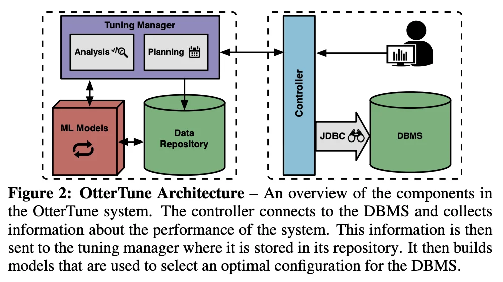
In short, you can divide the architecture into two halves. The client-side controller interacting with the runtime database and the server-side tuning manager which handles data collection, and the recommender systems. The server-side tuning manager has a repository of data from previous tuning-sessions as well. The goal is to make the database self-driving, as Andy Pavlo puts it. You want a database that is capable of automatically tuning itself when required.
Assumptions & Limitations
Before we discuss the details of the architecture, let’s quickly go over the assumptions made by the paper and it’s limitations.
Not “Completely” Self-Driving
There are certain real-world limitations that make this solution much more difficult to deploy in real world environments. For example, some of the “knobs” that the databases expose for tuning require the database to be restarted to actually have an effect. However, in the real-world, restarting prod databases especially are a major no-go. Further, due to specifications of how a company is deploying a database & the side-car’s attached to it, you might need a DBA to place limits on what knobs can be tuned and what knobs cannot be tuned. As such, OtterTune maintains a hardcoded blacklist of knobs that require restarts and also allows DBA’s to pass in extra knobs that they want to blacklist from tuning to guard against these issues.
Availability of a Near-Perfect Testing Environment
As we’ve highlighted already, the function we are trying to optimize depends heavily on the workload and instance configuration. To optimize a database in production, we assume that we have a copy of such a database that has near-identical configuration & load. In practice, this might be very difficult to acquire.
Database Design Must be Reasonable
In short,
Lastly, we also assume that the physical design of the database is reasonable. That means that the DBA has already installed the proper indexes, materialized views, and other database elements. There has been a considerable amount of research into automatic database design (Self-Tuning Database Systems: A Decade of Progress) that the DBA can utilize for this purpose. As discussed in Appendix C, we plan to investigate how to apply these same techniques to tune the database’s physical design.
The Architecture
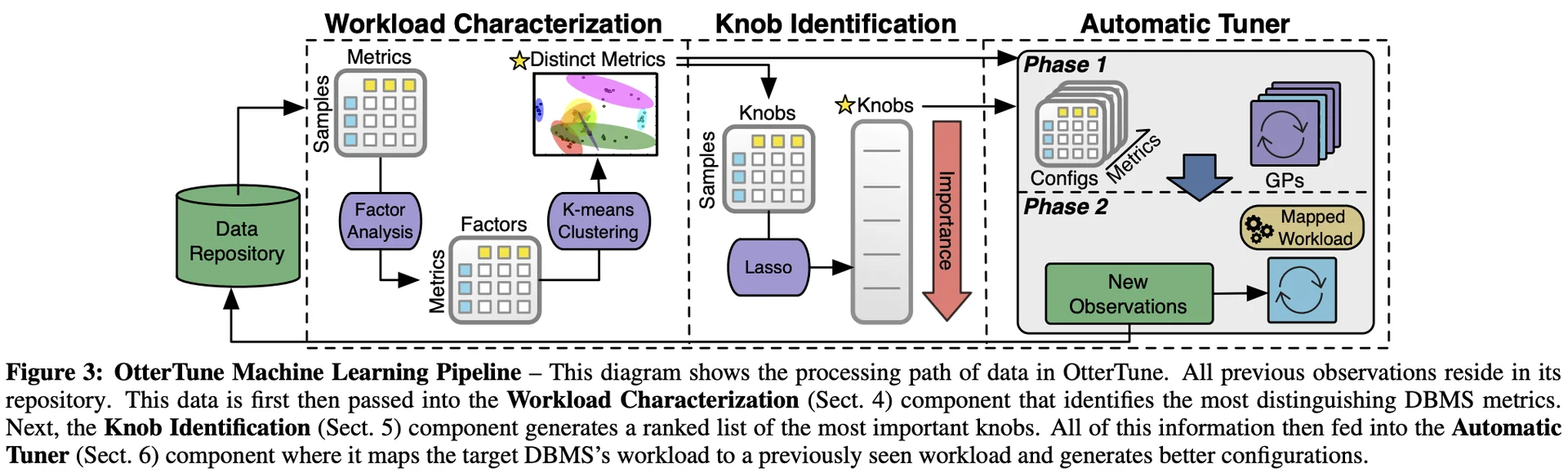
OtterTune works in three broad steps.
- Workload Characterization
- Knob Identification
- Automatic Tuning by Applying Knob configs
Workload Characterization
Perhaps the biggest problem that this paper, and OtterTune solve, is that of workload characterization. The ability to map previously unseen database workloads to known workloads. Running an optimization algorithm like gradient descent by collecting data many times by running a test workload on a test instance is not practically feasible. The costs would far outweigh the benefits. But by solving the problem of workload characterization, they unlock the ability to use a wealth of previously collected data for ML purposes.
But this is a difficult problem. When we say workload, we mean a collection of the following items at minimum:
- The instance configuration (This is easy)
- The RDBMS software & version (This is easy)
- A replay of the SQL queries the DBMS received (Difficult)
You can imagine that in an environment that supports both sharding & replication, this “workload” characteristic might have even more features to consider. How do we solve this complicated problem of taking two different workloads and getting an algorithm to judge their “similarity”? There were two main approaches considered.
Differing Approaches to Capture Similarity
Logical Analysis
You can attempt to analyze the workload at the logical level.
This means examining the queries and the database schema to compute metrics, such as the number of tables/columns accessed per query and the read/write ratio of transactions. These metrics could be further refined using the DBMS’s “what-if” optimizer API to estimate additional runtime information (AutoAdmin “What-if Index Analysis Utility), like which indexes are accessed the most often.
However, going back to the original problem, we want to be able to analyze how workload performance can be optimized by changing knobs. Given two differing workloads, changing knobs in each workload does not affect it’s logical definition. DBMSs execute queries by pushing the query through a query optimizer which may generate differing query plans with the slightest of changes to a query. The information we need cannot be captured by just examining the logical data.
Runtime Counter Analysis
The authors claim that a better approach is to use the DBMS’s internal runtime metrics to characterize how a workload behaves.
All modern DBMSs expose a large amount of information about the system. For example, MySQL’s InnoDB engine provides statistics on the number of pages read/written, query cache utilization, and locking overhead. OtterTune characterizes a workload using the runtime statistics recorded while executing it. These metrics provide a more accurate representation of a workload because they capture more aspects of its runtime behavior. Another advantage of them is that they are directly affected by the knobs’ settings. For example, if the knob that controls the amount of memory that the DBMS allocates to its buffer pool is too low, then these metrics would indicate an increase in the number of buffer pool cache misses.
There may be a little bit of manual effort into re-labelling the information presented by different DBMS software into the same label but it is doable. In practice, the main difference between the data collected by differing DBMS software lie in the granularity at which they capture and record this data. Some DBMS might capture it at the the level of individual components (per each buffer pool, for example) while others might only capture this information at the physical database level. However, in all instances, it is possible to aggregate this information at the physical database level for all modern DBMS software.
Personal Take: Why Not a Bit of Both?
While runtime metrics are very useful to judge the difference adjusting a knob makes, I believe it might be very easy for a knob change to drastically affect the query plan generated by the query optimizer for differing workloads. In these scenarios, a different query plan might suddenly make two previously similar workloads behave quite differently. True, in this scenario the runtime metrics should behave differently too but it is possibly something that can be explored.
Statistics Collection
Under the assumption that it is possible to get a near-identical copy of workload to work with, OtterTune starts tuning sessions by wiping the runtime counters clean, executing the workload and then grabbing the metrics right after the workload terminates. OtterTune grabs aggregated values to make this system work across multiple databases. But this also implies that it can only tune global to database knobs, instead of having more fine-grained control to specifics like each buffer pool’s size, etc.
Pruning Redundant Metrics
There may be a fair chunk of not-so-useful metrics in this proposed runtime statistics collection strategy. One reason is that certain knobs might have high correlation. The other is differing granularities for the same metric being reported.
For example, MySQL reports the amount of data read in terms of bytes and pages. … For example, we found from our experiments that the Postgres metric for the number of tuples updated5 moves almost in unison with the metric that measures the number of blocks read from the buffer for indexes.
This is essentially just the classic dimensionality reduction problem. They use one such technique, called factor analysis scikit-learn Documentation – Factor Analysis and k-means [scikit-learn Documentation – KMeans](http://scikit-learn. org/stable/modules/generated/sklearn.cluster.KMeans.html). This helps greatly reduce the search space for the ML algorithm & to also eliminate “noise” in the data. If you want a quick primer on dimensionality reduction, the paper does a great job here:
Given a set of real-valued variables that contain arbitrary correlations, FA reduces these variables to a smaller set of factors that capture the correlation patterns of the original variables. Each factor is a linear combination of the original variables; the factor coefficients are similar to and can be interpreted in the same way as the coefficients in a linear regression. Furthermore, each factor has unit variance and is uncorrelated with all other factors. This means that one can order the factors by how much of the variability in the original data they explain. We found that only the initial factors are significant for our DBMS metric data, which means that most of the variability is captured by the first few factors.
This is the detailed description from the paper:
The FA algorithm takes as input a matrix $X$ whose rows correspond to metrics and whose columns correspond to knob configurations that we have tried. The entry $X_{ij}$ is the value of metric $i$ on configuration $j$. FA gives us a smaller matrix $U$: the rows of $U$ correspond to metrics, while the columns correspond to factors, and the entry $U_{ij}$ is the coefficient of metric $i$ in factor $j$. We can scatter-plot the metrics using elements of the $i^{th}$ row of $U$ as coordinates for metric $i$. Metrics $i$ and $j$ will be close together if they have similar coefficients in $U$ — that is, if they tend to correlate strongly in $X$. Removing redundant metrics now means removing metrics that are too close to one another in our scatter-plot.
We then cluster the metrics via $k$-means, using each metric’s row of $U$ as its coordinates. We keep a single metric for each cluster, namely, the one closest to the cluster center. One of the drawbacks of using $k$-means is that it requires the optimal number of clusters ($K$) as its input. We use a simple heuristic [40] to fully automate this selection process and approximate $K$. Although this approach is not guaranteed to find the optimal solution, it does not require a human to manually interpret a graphical representation of the problem to determine the optimal number of clusters. We compared this heuristic with other techniques [55, 48] for choosing $K$ and found that they select values that differ by one to two clusters at most from our approximations. Such variations made little difference in the quality of configurations that OtterTune generated in our experimental evaluation in Sect. 7.
Factor Analysis
Let me explain that with a simple example. Let’s say we fix the workload and measure metrics $m_1, m_2, \cdots, m_n$ for configurations $c_1, c_2, \cdots, c_m$. Note that each configuration is in itself a vector of key value pairs for each individual knob that you can tune, but at the moment, let’s just give these vectors an ID and call each unique configuration ID a column. Our table looks like:
$$ \begin{array}{c|cccc} & c_1 & c_2 & \cdots & c_m \\ \hline m_1 & x_{11} & x_{12} & \cdots & x_{1m} \\ m_2 & x_{21} & x_{22} & \cdots & x_{2m} \\ \vdots & \vdots & \vdots & \ddots & \vdots \\ m_n & x_{n1} & x_{n2} & \cdots & x_{nm} \end{array} $$Factor analysis recognizes that we have an input of $m$ columns and tries to find a set of “underlying” factors with smaller cardinality that can represent these $m$ columns as linear combinations of the factors it identifies $\pm \text{unique variance}$. In short, let’s suppose we get $s \lt m$ factors $f_1, f_2, \cdots, f_s$. This essentially means that we can represent each of our original factors as some $c_i = \lambda_{i1}\eta_1 + \lambda_{i2}\eta_2 + \cdots + \lambda_i{s} + \epsilon_i$ where $\epsilon_i$ is the “unique” variance factor of metric $i$.
The factor coefficients are similar to and can be interpreted in the same way as the coefficients in a linear regression. Furthermore, each factor has unit variance and is uncorrelated with all other factors. This means that one can order the factors by how much of the variability in the original data they explain. We found that only the initial factors are significant for our DBMS metric data, which means that most of the variability is captured by the first few factors.
$k$-Means Clustering
Now, let’s suppose that the size of the factor set generated was exactly $s = 2$. If we plotted the two factors against each other now, each factor would be a data point in 2d space that we could run $k$-means on to identify similar metrics. With this, we can significantly reduce the number of metrics we want to use in our final optimization ML algorithm to reduce search space.
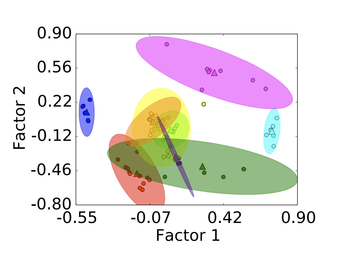
An interesting consequence of this clustering is that a lot of the useless metrics like output file name, etc. get mapped to the same cluster since their values don’t really depend on the configuration in any way whatsoever. The paper suggest providing some hints to the model to discard clusters containing parameters that we know for sure are useless.
From the original set of 131 metrics for MySQL and 57 metrics for Postgres, we are able to reduce the number of metrics by 93% and 82%, respectively. Note that OtterTune still collects and stores data for all of the DBMS’s metrics in its repository even if they are marked as redundant. The set of metrics that remain after pruning the FA reduction is only considered for the additional ML components that we discuss in the next sections.
Identifying Important Knobs
As mentioned before, this is a huge number of configurable variables or “knobs” that most modern RDBMS software expose for tuning, most of which are useless. So on the note of reducing search space, the next step we want to carry out is reducing the number of knobs we want to consider for tuning. The authors use a linear regression technique called Lasso regression (Lasso / Ridge / Elastic Net Regression) to find the knobs that have the highest correlation to the system’s overall performance.
OtterTune’s tuning manager performs these computations continuously in the background as new data arrives from different tuning sessions. In our experiments, each invocation of Lasso takes ∼20 min and consumes ∼10 GB of memory for a repository comprised of 100k trials with millions of data points. The dependencies and correlations that we discover are then used in OtterTune’s recommendation algorithms, presented in Sect. 6.
Lasso Regression
Lasso regression is used to perform regression but with slightly increased bias in exchange for reduction in variance. This technique is particularly useful when the variables we use for tuning might contain several useless variables which do not contribute any variance to the parameter we are predicting by tuning their weights to 0.
The paper in particular, uses a version of lasso called the Lasso path algorithm as described in The Elements of Statistical Learning.
The algorithm starts with a high penalty setting where all weights are zero and thus no features are selected in the regression model. It then decreases the penalty in small increments, recomputes the regression, and tracks what features are added back to the model at each step. OtterTune uses the order in which the knobs first appear in the regression to determine how much of an impact they have on the target metric (e.g., the first knob selected is the most important).
Before OtterTune computes this model, it executes two preprocessing steps to normalize the knobs data. This is necessary because Lasso provides higher quality results when the features are (1) continuous, (2) have approximately the same order of magnitude, and (3) have similar variances. It first transforms all of the categorical features to “dummy” variables that take on the values of zero or one. Specifically, each categorical feature with n possible values is converted into n binary features. Although this encoding method increases the number of features, all of the DBMSs that we examined have a small enough number of categorical features that the performance degradation was not noticeable. Next, OtterTune scales the data. We found that standardizing the data (i.e., subtracting the mean and dividing by the standard deviation) provides adequate results and is easy to execute. We evaluated more complicated approaches, such as computing deciles, but they produced nearly identical results as the standardized form
To capture relationships between variables, such as dependencies between memory allocations (since maximizing every individual knob that allocated memory would lead to trashing from the system running out of memory), we introduce polynomial terms in the equation. The output of the lasso path algorithm is a list of all knobs, sorted in the amount of impact they have on a target metric. Now we need to figure out how many terms of the equation we want to keep and how many to discard. We can obviously consider binary searching the “optimal” point, but the paper suggests using an incremental approach where OtterTune dynamically increases the number of knobs used in a tuning session over time. They claim this to be effective in other optimization algorithms as well and this is likely fine since the number of knobs we will get an optimal prefix with is likely pretty small.
Automated Tuning
Now that we’ve gotten a lot of the “pre-processing”, if you want to call it that, parts out of the way, we can move on to the fun stuff. When tuning a new workload, OtterTune divides the tasks into two broad sections.
- Workload Mapping $\to$ Tries to map the new workload to some existing workload data in the database.
- Configuration Recommendation $\to$ Tries to use the data points from the “similar” workload identified in the previous steps and then adds new data points from the new workload by trading off exploration vs exploitation using Gaussian Regression. (Which I will hopefully write a blog about in the future. I can understand the overarching ideas, but the math is black magic to me at the moment :)
Workload Mapping
The first step that OtterTune does when given a new optimizing task, is to run a few replays of the workload on a few different previously seen configurations and records the metrics of the run. Once this is done, it tries to match the previously seen workload that has the most similar metric readings for the configurations tested. As we run more test runs on different configurations, the quality of the match made by OtterTune increases, which is what we’d expect to see. The below describes this matching process in more detail:
For each DBMS version, we build a set $S$ of $N$ matrices — one for every non-redundant metric — from the data in our repository. Similar to the Lasso and FA models, these matrices are constructed by background processes running on OtterTune’s tuning manager (see Sect. 3). The matrices in $S$ (i.e., $X_0, X_1, \cdots. X_{N−1}$) have identical row and column labels. Each row in matrix $X_m$ corresponds to a workload in our repository and each column corresponds to a DBMS configuration from the set of all unique DBMS configurations that have been used to run any of the workloads. The entry $X_{m,i,j}$ is the value of metric $m$ observed when executing workload $i$ with configuration $j$. If we have multiple observations from running workload $i$ with configuration $j$, then entry $X_{m,i,j}$ is the median of all observed values of metric $m$.
The workload mapping computations are straightforward. OtterTune calculates the Euclidean distance between the vector of measurements for the target workload and the corresponding vector for each workload $i$ in the matrix $X_m$ (i.e., $X_{m,i,:}$). It then repeats this computation for each metric $m$. In the final step, OtterTune computes a “score” for each workload $i$ by taking the average of these distances over all metrics $m$. The algorithm then chooses the workload with the lowest score as the one that is most similar to the target workload for that observation period.
That was the crux of it. Essentially compute the similarity score between our new workload and any of the previously seen workloads by computing euclidean distance between performance metrics for both the workloads on the same configuration. To make this work correctly you’ll need to also do some normalization / binning which is described below.
Before computing the score, it is critical that all metrics are of the same order of magnitude. Otherwise, the resulting score would be unfair since any metrics much larger in scale would dominate the average distance calculation. OtterTune ensures that all metrics are the same order of magnitude by computing the deciles for each metric and then binning the values based on which decile they fall into. We then replace every entry in the matrix with its corresponding bin number. With this extra step, we can calculate an accurate and consistent score for each of the workloads in OtterTune’s repository.
Configuration Recommendation
OtterTune uses a regression technique called Gaussian Process Regression which they claim to be the state-of-the-art technique with power approximately equal to that of deep networks. I know too little about ML & the math behind how Gaussian Process Regression works is still black magic for me, so I’ll try to give the intuitive understanding that I got from reading A Visual Exploration of Gaussian Processes - Distill.
Gaussian Processes (A very high level overview)
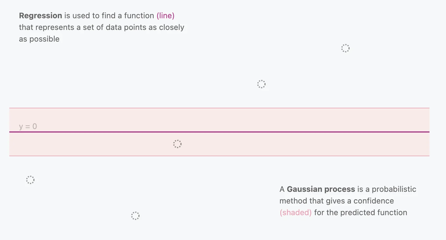
Regression is just a term we give to techniques used to find a function that represents the ‘best-fit’ for a set of data points as closely as possible. We usually define some notion of cost to minimize and regression minimizes this cost, giving us our ‘best-fit’ function.
Gaussian Processes are a probabilistic method that gives a confidence interval for the predicted function. The mean of the distribution would be the “best-fit” line, but the variance would help us gauge our confidence in a given prediction.
There are infinitely many functions that can fit your data. Gaussian processes offer an elegant solution to this problem by assigning a probability to each of these functions.
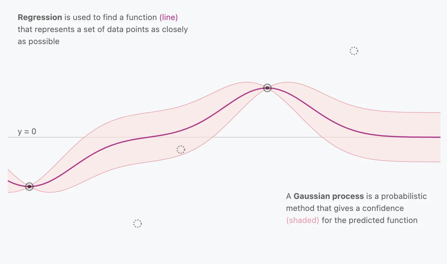
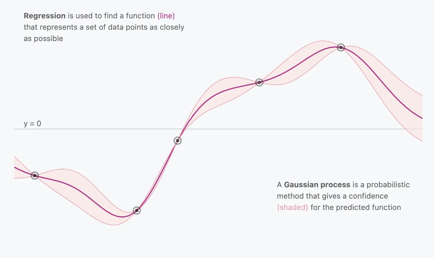
You’ll also notice that at locations where multiple data points are present, the distribution is very narrow, signifying high confidence. On the other hand, near the horizontal ends you’ll see the distribution widen, signifying lower confidence, which is what we want to see.
Searching with GPs
The paper also claim that GPs are able to provide a theoretically justified way to trade off exploration (acquiring new knowledge) and exploitation (making decisions based on existing knowledge).
Remember that OtterTune has mapped the new workload to some existing previously seen workloads which has already recorded it’s execution on multiple different configurations. OtterTune starts from these values and then adds the new data points collected by actually running the new workload.
Since the mapped workload might not exactly match the unknown workload, the model’s predictions are not fully trusted. To address this, we increase the noise parameter variance for all untried points in the GP model by adding a ridge term to the covariance. We also add a smaller ridge term for each configuration selected. The claim is that this approach helps in handling variability in virtualized environments where DBMS metrics like throughput and latency can vary between observations.
In the context of our proposed solution:
Exploration $\to$ Search an unknown region in its GP $\to$ Run the workload on far-away from GP distribution configuration, possibly adjusting several config parameters at the same time. (Remember, this GP is $m$-d space, where $m$ is the number of knobs to tune.) This can be particularly useful when OtterTune is trying to change knob values where the upper or lower limit for the knob’s best value might depend on the underlying hardware. (Ex: Total memory available.)
Exploitation $\to$ Select a configuration that is near the best configuration in its GP $\to$ Run the workload on a configuration that is somewhere close to where the GP has high confidence, to confirm & slightly improve performance with fine-tuned adjustment.
Which of these two strategies OtterTune chooses when selecting the next configuration depends on the variance of the data points in its GP model. It always chooses the configuration with the greatest expected improvement. The intuition behind this approach is that each time OtterTune tries a configuration, it “trusts” the result from that configuration and similar configurations more, and the variance for those data points in its GP decreases. The expected improvement is near-zero at sampled points and increases in between them (although possibly by a small amount). Thus, it will always try a configuration that it believes is optimal or one that it knows little about. Over time, the expected improvement in the GP model’s predictions drops as the number of unknown regions decreases. This means that it will explore the area around good configurations in its solution space to optimize them even further.
Gradient Descent
The output of the GP is the function, in this case a $m$ dimensional surface, that it believes models the function for our new workload the best. Once we have this surface, we have finally reduced our problem to the standard ML problem we described all those ages back :)
There are two types of configurations in the initialization set: the first are the top-performing configurations that have been completed in the current tuning session, and the second are configurations for which the value of each knob is chosen at random from within the range of valid values for that knob. Specifically, the ratio of top-performing configurations to random configurations is 1-to-10. During each iteration of gradient descent, the optimizer takes a “step” in the direction of the local optimum until it converges or has reached the limit on the maximum number of steps it can take. OtterTune selects from the set of optimized configurations the one that maximizes the potential improvement to run next. This search process is quick; in our experiments OtterTune’s tuning manager takes 10– 20 sec to complete its gradient descent search per observation period. Longer searches did not yield better results.
Similar to the other regression-based models that we use in OtterTune (see Sects. 5.1 and 6.1), we employ preprocessing to ensure that features are continuous and of approximately the same scale and range. We encode categorical features with dummy variables and standardize all data before passing it as input to the GP model.
Once OtterTune selects the next configuration, it returns this along with the expected improvement from running this configuration to the client. The DBA can use the expected improvement calculation to decide whether they are satisfied with the best configuration that OtterTune has generated thus far.
Results
OtterTune vs iTuned
Refer to the paper to obtain a more comprehensive overview of the test-suite and results. In short, the major contribution OtterTune brought is the ability to re-use previously seen workloads to tune new unseen workloads. And as such, they compare the performance of OtterTune with, iTuned a similar automatic DBMS tuning software that uses GPs. However, instead of starting from previously seen data, iTuned uses a stochastic sampling technique called Latin Hypercube Sampling to generate an initial set of 10 DBMS configurations that are executed at the start of the tuning session. Optimizing for the 99th percentile latency metric, they obtain the following results:
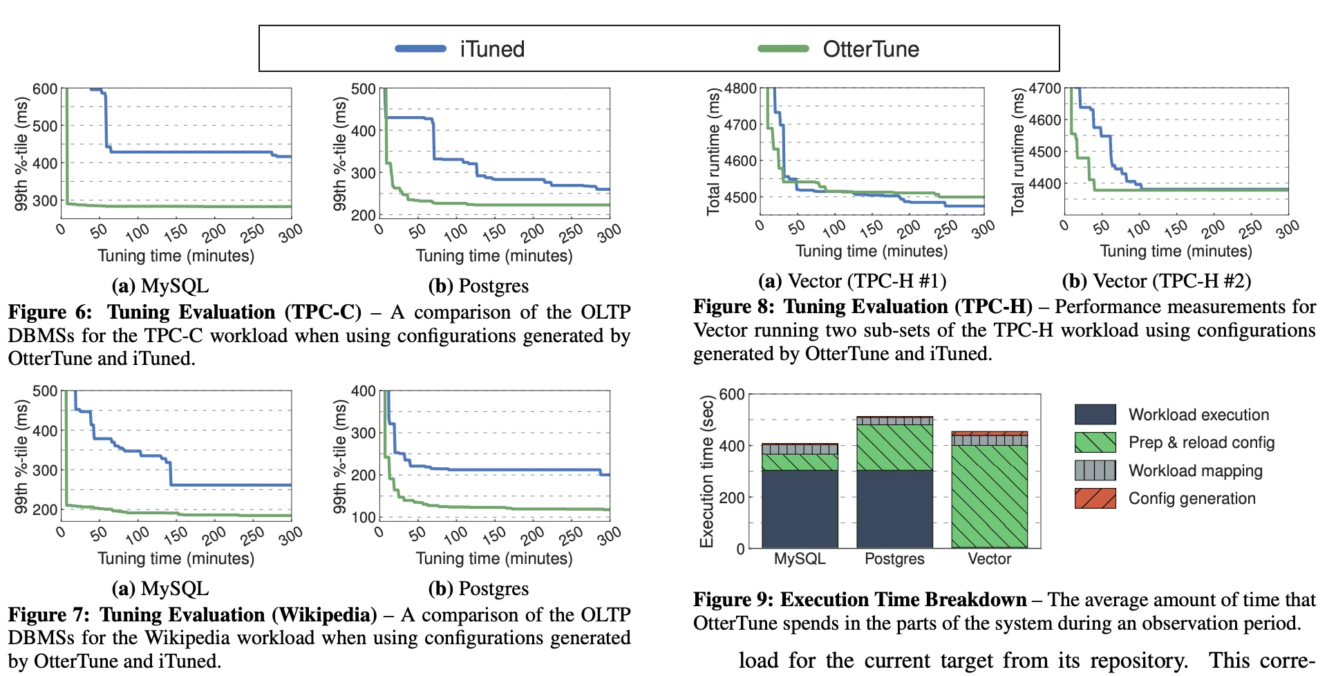
In general, we observe that OtterTune is able to converge to it’s optimal configuration much faster than iTuned. It also outperforms it by a significant margin on OLTP workloads. In contrast, you’ll notice that the gap is nowhere near as pronounced in OLAP workloads. It even seems to lose to iTuned on the OLAP workload. The authors claim that this difference is mainly due to the fact that the OLAB database, Vector exposes much less values for tuning and is less permissive on what values are allowed to be set too. This makes tuning Vector a much simpler problem than MySQL or Postgress, limiting the room for improvement.
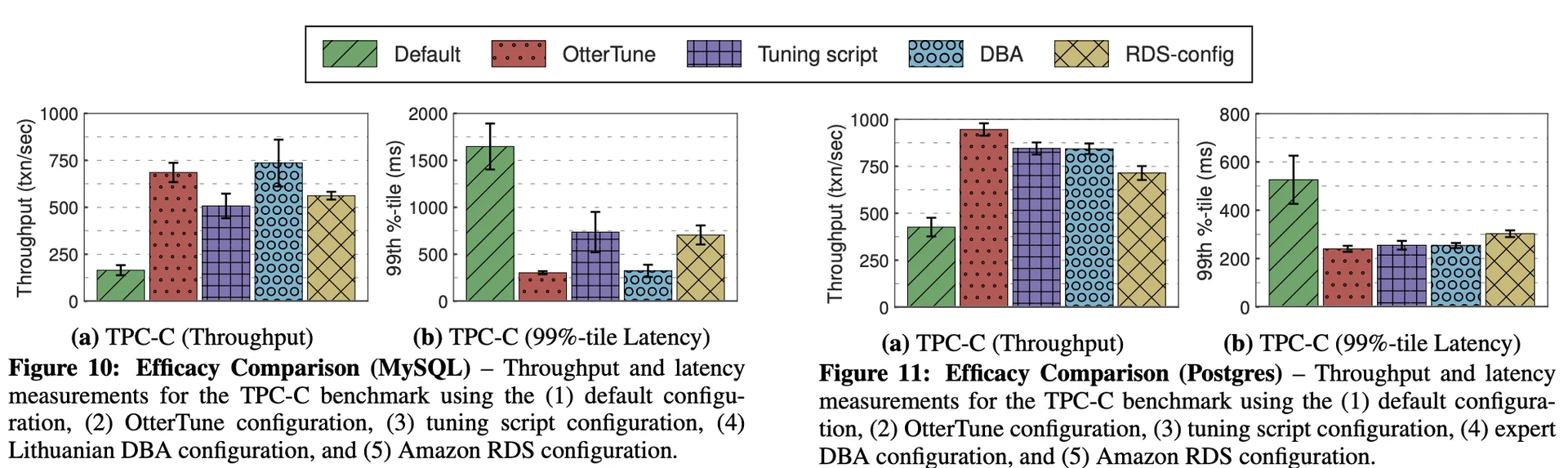
OtterTune vs DBAs & Other Usual Tuning Strategies
Conclusion
We presented a technique for tuning DBMS knob configurations by reusing training data gathered from previous tuning sessions. Our approach uses a combination of supervised and unsupervised machine learning methods to (1) select the most impactful knobs, (2) map previously unseen database workloads to known workloads, and (3) recommend knob settings. Our results show that OtterTune produces configurations that achieve up to 94% lower latency compared to their default settings or configurations generated by other tuning advisors. We also show that OtterTune generates configurations in under 60 min that are comparable to ones created by human experts.