Profiling a Program
Interactive Graph
Table of Contents
Profiling Programs
Any examples shown below are from running the profiler on a small piece of code I wrote to test the Goldbach Conjecture, usually run until $N \leq 5000$. Sample Goldbach Conjecture test program to profile
time
The simplest way to profile a program is to perhaps run the Linux time command, which simply executes the given program and returns 3 values.
real- The elapsed real time between invocation and terminationuser- The amount of time spent by the calling process and its children executing instructions in user spacesystem- The amount of time spent by the kernel in kernel space performing tasks on behalf of the calling process and it’s children
It’s the quickest and simplest way to profile a program, however, it gives very little information to go off of. Which part of the code is the bottleneck? Are algorithms or memory usage the bottleneck?
Program Instrumentation A natural idea to benchmark code is to insert a tiny chunk of code just before and after the function call site, like so:
tick()foo()tock()Tick and tock are small bits of code that log information like CPU time or wall-clock time and other state info before and after the function call. We call this “Instrumenting” the code. This would essentially give us the time each function in our code takes to execute but this is understandably laborious to do, especially in large codebases.
The obvious solution here is to offload this manual work to the compiler. There are two ways to do compile-time program instrumentation.
- The
-pgflag - We discuss this in great detail in the section about thegprofprogram.- The
-finstrument-functionsflag - This essentially allows us to write our own customtickandtockfunctions which the compiler automatically instruments every function in our code with. We can optionally exclude functions as well. Details can be found in this Jacob Sorber video.
gprof
The gprof tool relies on compile-time program instrumentation tactics to produce an execution profile of a program.
How to use?
- Compile and link the source code with the
-pgflag. - Run the generated executable normally. If your program takes some input, it might be worthwhile to run the program on both slow and fast cases.)
- Run
gprof a.out gmon.out > fast-tc.txt. Here,a.outis the name of your executable, andgmon.outis the name of the file created upon initial execution. Since you might be profiling different source codes/test cases/compiler options it’s good practice to pipe the output to well-named files.
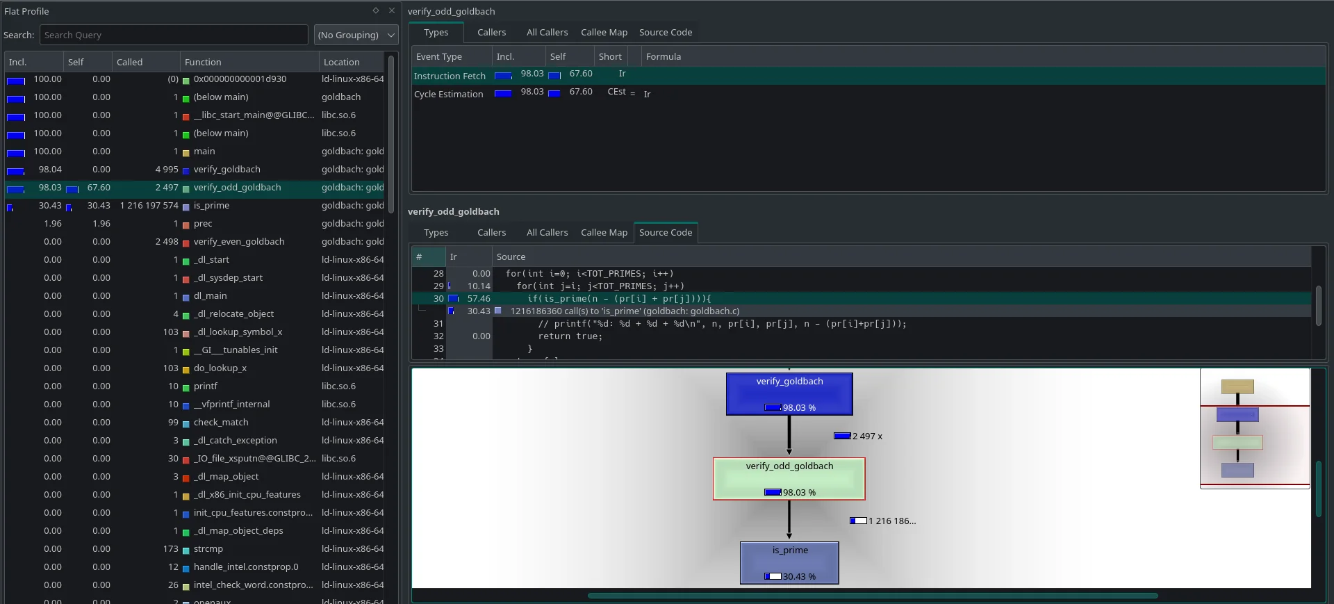
It provides two main information views. A Flat Profile and a Call Graph.
- Flat Profile: It shows how much time our program spends in each function and the number of times it is called. Gives concise information about which functions were the big bottlenecks in the program.
Flat profile:

Each sample counts as 0.01 seconds.
  %   cumulative   self              self     total
 time   seconds   seconds    calls  ms/call  ms/call  name
 77.01      2.11     2.11     2497     0.85     1.05  verify_odd_goldbach
 18.98      2.63     0.52 1216197574     0.00     0.00  is_prime
  4.01      2.74     0.11        1   110.00   110.00  prec
  0.00      2.74     0.00     4995     0.00     0.53  verify_goldbach
  0.00      2.74     0.00     2498     0.00     0.00  verify_even_goldbach
Most of the columns are pretty self-explanatory. self seconds is the amount of time spent in that function call frame and calls is the number of times it was called. total ms/call is the total amount of time spent in the functions call frame + its descendants per call.
- Call Graph: For some function $f$, it shows the functions which called it and which other functions it called, and how many times they were called. It also provides an estimate of how much time was spent in the subroutines of each function. This can suggest places where you might try to eliminate function calls that use a lot of time.
index % time    self  children    called     name
                                                 <spontaneous>
[1]    100.0    0.00    2.74                 main [1]
                0.00    2.63    4995/4995        verify_goldbach [2]
                0.11    0.00       1/1           prec [5]
-----------------------------------------------
                0.00    2.63    4995/4995        main [1]
[2]     96.0    0.00    2.63    4995         verify_goldbach [2]
                2.11    0.52    2497/2497        verify_odd_goldbach [3]
                0.00    0.00    2498/2498        verify_even_goldbach [6]
-----------------------------------------------
                2.11    0.52    2497/2497        verify_goldbach [2]
[3]     96.0    2.11    0.52    2497         verify_odd_goldbach [3]
                0.52    0.00 1216186360/1216197574     is_prime [4]
-----------------------------------------------
                0.00    0.00   11214/1216197574     verify_even_goldbach [6]
                0.52    0.00 1216186360/1216197574     verify_odd_goldbach [3]
[4]     19.0    0.52    0.00 1216197574         is_prime [4]
-----------------------------------------------
                0.11    0.00       1/1           main [1]
[5]      4.0    0.11    0.00       1         prec [5]
-----------------------------------------------
                0.00    0.00    2498/2498        verify_goldbach [2]
[6]      0.0    0.00    0.00    2498         verify_even_goldbach [6]
                0.00    0.00   11214/1216197574     is_prime [4]
-----------------------------------------------
Index by function name

   [4] is_prime                [6] verify_even_goldbach    [3] verify_odd_goldbach
   [5] prec                    [2] verify_goldbach
Reading this is simple and mostly self-explanatory as well. Each function is assigned a unique id number. Now, in each entry of the table, the line containing the index id on the leftmost column is the current function. Every line in the entry above this line is a function that called the current function and everything below it is a function that was called by the current function.
The good part about it is that it is extremely fast and provides some worthwhile profile information about the program.
The primary issue with gprof is that it requires the original executable to be instrumented, which means changing the original source code. To be more specific, the extra instrumenting functions called before and after every function call site add extra overhead to the function call. This can skew the profile information returned, especially when dealing with small fast functions which are called many many numbers of times.
To not have to deal with skewed results due to instrumentation, we might consider using a different method for profiling, sampling profiling
valgrind --tool=callgrind
callgrind is similar to gprof in the sense it also provides a flat profile and call graph except it is a lot more visually appealing and because it runs on valgrind, it can capture a lot more detailed information about the executable. However, this extra information and visual appeal come at a major cost, running the program on valgrind is computationally much more expensive.
For context, compiling the instrumented -pg program and executing it with no optimizations took 14.563 seconds total as measured by time. Running it using callgrind on the other hand took a whopping 3 mins and 15 seconds total. Running with O3 optimizations turned on, we find that -pg takes 0.622 seconds to run while callgrind took 1 min and 1 second.
callgrind works by emulating a CPU and getting samples of the program execution at different points in time. This slows down the program overall but slows down all parts by relatively the same amount so the final ratios/percentages it returns are fairly accurate and not skewed by any external overheads. We can use tools like kcachegrind to present the output of callgrind in a very visually pleasing manner. kcachegrind provides us with all the information that gprof does and more. We also get to see a line-by-line analysis of the source code showing what percentage of time a particular instruction/line of code is executed.
perf
You can run perf using the command sudo perf stat ./goldbach. It uses a type of sampling which relies on certain specific hardware registers used for profiling. Sample output looks something like this,
Note: Could not run it for goldbach because it was unable to track cache-misses, branch-misses, instructions, cycles, etc. due to lack of hardware support. (Unsure if it is due to VM or AMD CPUs)
Performance counter stats for 'dd if=/dev/zero of=/dev/null count=1000000':

            5,099 cache-misses             #      0.005 M/sec (scaled from 66.58%)
          235,384 cache-references         #      0.246 M/sec (scaled from 66.56%)
        9,281,660 branch-misses            #      3.858 %     (scaled from 33.50%)
      240,609,766 branches                 #    251.559 M/sec (scaled from 33.66%)
    1,403,561,257 instructions             #      0.679 IPC   (scaled from 50.23%)
    2,066,201,729 cycles                   #   2160.227 M/sec (scaled from 66.67%)
              217 page-faults              #      0.000 M/sec
                3 CPU-migrations           #      0.000 M/sec
               83 context-switches         #      0.000 M/sec
       956.474238 task-clock-msecs         #      0.999 CPUs utilized

       0.957617512  seconds time elapsed
The output is useful in determining which type of operation is becoming the major bottleneck in the program. perf report can be used to get the flat profile and call graph for the program as well.
We can quickly determine if the program is parallelized or not (0.999 CPUs utilized for example, certainly means that the program is not parallelized.), and also quickly determine what is severely limiting the program, cache misses or instruction execution. Many times, memory accesses are a limiting factor due to the slow speeds of memory, and perf can quickly provide you statistics about that.
Hardware sampling is also not the most accurate it can be. It’s better than instrumentation but not as accurate as valgrind either.
PIN, PAPI, VTune, etc.
A plethora of other tools exists as well. PIN is a fairly advanced tool that works by instrumenting binary code. PAPI is an API that helps profile-specific sections of code. VTune is a similar profiling tool provided by Intel that has received high praise.
Profiling via Time Measurement vs Stack sampling
While profiling by measuring the time of execution of different parts of the program is taught as the mainstream way to locate “hotspots” in code, there’s another very interesting idea one might use to locate bottlenecks. Most of the following content comes from what Mike Dunlavey pitches on multiple Stack Overflow posts. The following is long but definitely worth going over once.
- Why not use
gprofand similar tools for profiling? - How to profile code using stack samples and why is it often better?
- A very simple explained example workflow
- A more complex example explained
A brief of what the above posts try to convey
A lot of profiling software look at the correct data, they take samples of the call stack and process data which contains enough info to infer where the hotspots in the code are, but most end up “summarizing” the data and lose a lot of valuable information in this process.
Let the cloud here represent the bottleneck,
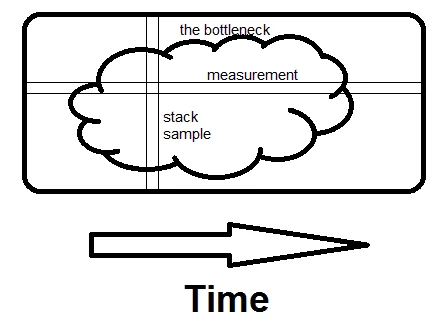
The measurement in the profile tells us what function took up a major chunk of the time but it fails to give a clear understanding of why? and it is this information that we are trying to hang on to. Without knowing the “why?” it’s as good as an educated guess when trying to identify the hotspots. When sampling call stacks, we get a detailed picture of the sequence of events leading up to something and get a much better idea of why something might be eating up a lot of time and what specifically to address.
This specific information is often lost when profilers end up summarizing the data for end users to see. To quote,
Measurement is horizontal; it tells you what fraction of time specific routines take. Sampling is vertical. If there is any way to avoid what the whole program is doing at that moment, and if you see it on a second sample, you’ve found the bottleneck. That’s what makes the difference - seeing the whole reason for the time being spent, not just how much.
The stack samples don’t just tell you how much inclusive time a function or line of code costs, they tell you why it’s being done, and what possible silliness it takes to accomplish it.
References
These notes are quite old, and I wasn’t rigorously collecting references back then. If any of the content used above belongs to you or someone you know, please let me know, and I’ll attribute it accordingly.