Last time we discussed A Deep Dive into the Knapsack Problem. Today, we’ll look at three more interesting problems with cool Dynamic Programming solutions.

Shortest Reliable Path

Consider the following dispatch problem. Often when trying to schedule deliveries of goods, it is not good enough to only determine the shortest path from source to destination. One needs to also take into account the number of points at which the goods must switch transport vehicles. This could have an effect on the quality of goods received. We can have similar applications in networking where we do not want to switch edges multiple times. In these cases, we try to solve a slight variation of the shortest path problem.

The shortest reliable path problem asks the following question, “Given a graph $G$ with weighted edges, what is the shortest path from location $s$ to location $t$ such that the path consists of at most k-edges?”

We can solve this problem using dynamic programming.

The DP solution

Let’s think about the following recurrence. If I know what the shortest path to some vertex $v$ is using $i$ edges, I can just go over all my edges again in a “relaxation” step and find out what the shortest path to vertex $v$ is using $i+1$ edges. We have identified our subproblem!

Let’s define $dp[i][j]$ as the shortest path to reach vertex $i$ using just $j$ edges.

1. Number of subproblems

   Notice that we have $|V|$ number of vertices and will have to compute the answer for $i:1\to k$ edges. Therefore we will have $|V|k$ subproblems. $k$ can be around $m$. This would then require $O(|V|m)$ problems solved.

2. Finding how to brute force the solution to some subproblem state

   To go from knowing the shortest paths using $i$ edges, to know the solution when using $i+1$ edges, we will have to “relax” all the edges once. We can solve all the subproblems for some number of edges $k'$ by just iterating over the entire edge list in $O(m)$

3. Finding the recurrence

   As mentioned previously, relaxing all edges will net us the desired result.

   We can write the recurrence as

   $$ dp[v][i] = min_{(u,v)\in E}(dp[u][i-1]+l(u,v), dp[v][i]) $$

   Notice that this implies that we initially consider all distances from $v$ to any other vertex as $\infty$.

4. Figuring out DAG structure

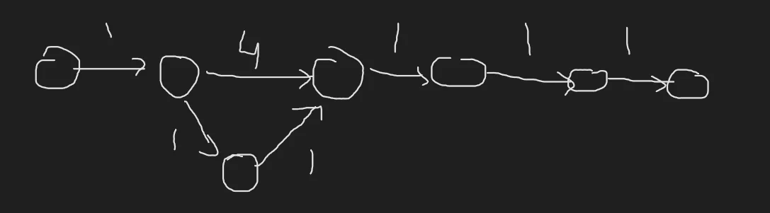
   We can visualize this as a simple linear chain. We solve the problem for all vertices using $i+1$ edges in one go. So we can just think of it as a linear chain going from $i=1\to 2 \to 3\to \dots \to k$ edges.

5. Completing the solution

   Armed with all the information we need, all we need to do now is calculate the final solution. Since we’re computing $k$ problems in $O(m)$ iterations each, the solution has overall $O(km)$ complexity where $m = |E|$. In the worst case when $k \to m$ we can have $O(m^2)$ complexity.

A tighter bound

Notice that our solution is very similar to the Bellman-Ford algorithm. It’s because Bellman-Ford and our algorithm work on the same principle. Both the algorithms solve the very same subproblems. But notice that any spanning tree of our graph will connect all vertices and this implies that there will always be a path between two vertices using just $n-1$ vertices. This means repeating our algorithm $n-1$ times will converge at the optimal shortest distance solution.

From this fact, we can naturally conclude that the bound on the value of $k$ is $|V|$. Therefore our solution will not have $O(m^2)$ complexity as we can bound $k = min(k, |V|-1)$. This gives our algorithm a better runtime of $O(|V||E|)$.

1D Row Optimization

Notice that again, we are computing the answer for all $v \in V$ using $i$ edges using the answer for $i-1$ edges. This means that we in fact do not need to store the solution for all $O(|V|k)$ subproblems. Simply storing the answer for $O(|V|)$ subproblems would be enough.

Hence we can optimize it to just using 1 row.

Code

The code for this DP solution is quite beautiful and short. Vector d stores the DP values for any given state. Here, we assume the graph is stored in edge list representation. e is the edge list.

vector<int> d (n, INF);
d[v] = 0;
for (int i=0; i<min(k, n-1); ++i)
    for (int j=0; j<m; ++j)
        if (d[e[j].a] < INF)
            d[e[j].b] = min (d[e[j].b], d[e[j].a] + e[j].cost);

An alternate Greedy + DP solution

Dijkstra is a greedy algorithm that computes the shortest paths solution in $O(ElogV)$ with the help of a priority queue implementation using some heap. Notice that we can modify how the heap stores its top element and eliminate some skipping to arrive at a solution for the shortest reliable paths problem!

Let’s say I said that my new criteria for highest priority were a pair $(i, dis[v])$. In this notation, I first sort priority using $i$. The pair with the lowest $i$ is given the highest priority. Once sorted by $i$, we assign priority based on the smallest $dis[v]$.

Our claim

I claim that with this additional bookkeeping, we will be able to solve this problem once we eliminate a speedup check in the original Dijkstra.

Let’s think about what this additional bookkeeping is doing. By enforcing this constraint, we are essentially saying that we must first update all reachable vertices using the smallest number of edges $i$. So we are just simply running Dijkstra for a more constrained graph. This means that I will be able to compute the solution using $i$ edges.

However, Dijkstra skips over all the nodes already visited. This is essential in keeping the complexity down. Consider this case.

We will not be able to update the third node from the left do distance 3 once it has already been processed for reachability using 2 edges. Hence we will have to eliminate this skipping and force the algorithm to process new vertices again.

How is this different from the previous solution?

Notice that in the previous solution, for any randomized sparse graph, we would, in the beginning, be iterating over many edges that are from the reach of the source node using a small number of edges. This is redundant work that we were doing. Here, we are only iterating over the edges that are reachable.

The complexity of this solution

Assuming we are using a priority queue, our solution has the worst time runtime of $O(kElogV)$. However, notice that because we are not iterating over every edge on every iteration, for sparse graphs where $k$ is small, we might have a better/faster runtime using this solution.

Floyd Warshall

The problem is as follows, “Given a graph G, find the shortest distance between all pairs of points.”

Notice that we can compute the answer to this problem simply by running Dijkstra $|V|$ times. This would have an overall runtime of $O(|V||E|log|V|)$. For dense graphs, the complexity might reach $O(n^3logn)$ where $n = |V|$. We also require at the very minimum, a binary heap implementation of a priority queue.

Further, this solution will not work if the graph contains any negative edge weights.

The DP Solution

The first step to solving it with DP is identifying a subproblem. Let’s say I order my nodes in some arbitrary fashion. This implies that my nodes are always in some order and the concept of “first k nodes” can be applied to them. Now, I can define by DP state as follows:

Let $dp[i][j][k]$ represent the length of the shortest path from nodes $i \to j$ using just $k$ nodes as intermediaries. Notice that now, we can define a recurrence between subproblems as follows:

Let’s see what this means. When computing the shortest distance between any two nodes $i, j$ using $k$ intermediary nodes, we assume that we know the optimal solution to the distance between them when using just $k-1$ intermediaries.

If these subproblems have been solved, then when computing the shortest distance between $i,j$ using $k$ intermediaries, the question essentially boils to asking “Should we include intermediate node $k$ in the shortest path?”

To answer this, we check what the shortest path from $i \to k$ is and $k \to j$ is using $k-1$ intermediate nodes. If the sum of these distances is lesser than the min computed so far, we can include node $k$. Notice that we are simply including 1 node. Therefore our computation for the DP state will be correct.

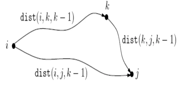
This is a visual representation of the sub-problem we’re attempting to solve.

Now for the base case, the distance between any two nodes using 0 intermediary nodes will be $\infty$ when they’re not connected and $l(u,v)$ when they are connected. It’s essentially the adjacency matrix representation of the graph with disconnected vertices marked with $\infty$.

Time complexity

We have $i\cdot j \cdot k$ subproblems to solve and each sub-problem takes $O(1)$ computation to solve.

Therefore overall time complexity of our algorithm will be $O(n\times n\times n) = O(n^3)$ . Here $n = |V|$.

Space complexity

Notice that naively, we must store the computation for $O(n^3)$ subproblems and hence require $O(n^3)$ space. However, notice that we can do something very similar to 1D row optimization. Notice that for computing all subproblems with DP state $k$, we only require the solution of all-pairs shortest paths using $k-1$ intermediaries. This means we only need to store $O(n^2)$ solutions at any point in time. Hence we can reduce the space complexity down to $O(n^2)$.

Code

Again, as with most DP solutions, the code is quite short and sweet :)

for (int k = 0; k < n; ++k) {
    for (int i = 0; i < n; ++i) {
        for (int j = 0; j < n; ++j) {
            d[i][j] = min(d[i][j], d[i][k] + d[k][j]); 
        }
    }
}

Independent Set in a tree

The problem we’re trying to solve here is as follows, “Given a tree G, find the largest independent set of vertices belonging to the tree. Here, we define a subset of vertices $S$ of $V$as independent if there are no edges belonging to G which connect any two pair of vertices in the subset $S$.”

From the definition of “independent set”, we can easily conclude that the set $S$ must be a bipartite subset of $G$. However, notice that any bipartite coloring won’t do. More specifically, a bipartite coloring where we color one node then skip it’s children and proceed won’t do.

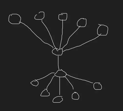
This is a simple counter case to that solution. We require both the lumps of vertices and the bottom and the top for the optimal solution. Notice that this hints us towards the sub-problem we require to solve.

The DP Solution

We can define our sub-problem as follows, “Should we include node $u$ in the answer or not?” To further this and make this more useful, we can define a DP state as follows: “How many nodes would I get in my optimal matching if I included node $u$ in the subset?”

If our DP stores this, notice that every node $u$ is the root of some subtree. This means we can calculate the answer for each subtree of $G$ and the answer will be the $DP$ state for the root of the tree.

Now, how do we find the recurrence?

This can be done greedily.

Notice that if we include $u$ in the answer, we cannot include any child of $u$. The next best option is to include the grandchildren (children of children) of $u$.

Notice that this is optimal. Because every $DP$ state stores some positive quantity and not choosing to include a grandchild would imply we missed a chance to increase the value. Further, each DP state is only dependent on its children and grandchildren. Hence this decision does not affect future DP states.

If we do not include $u$ in the answer, then we must pick all its children. The reasoning for this is the same as the above.

Now, we have a recurrence.

With our $DP$ state defined as

we can define the recurrence as follows

$DP[i] = max(1 + \sum_{grandchildnren \ x} DP[x] , \sum_{children \ y} DP[y])$

The first term is the maximum answer attainable when including $i$. The second term is the maximum attainable when not including $i$. These are the only two conditions possible.

Time complexity

Notice that we have $O(n)$ where $n = |V|$ subproblems to solve for and each subproblem takes $O(1)$ complexity. Therefore the overall time complexity of our algorithm is $O(|V|)$.

Space complexity

We have $O(n)$ subproblems to solve. This gives us a space complexity of $O(n)$.

References

These notes are old and I did not rigorously horde references back then. If some part of this content is your’s or you know where it’s from then do reach out to me and I’ll update it.

1. Professor Kannan Srinathan’s course on Algorithm Analysis & Design in IIIT-H