The Black-Scholes-Merton Equation
Interactive Graph
Table of Contents
This single equation spawned multi-trillion dollar industries and transformed everyone’s approach to risk.
$$ \frac{\partial V}{\partial t} + rS\frac{\partial V}{\partial S} + \frac{1}{2}\sigma^2S^2\frac{\partial^2V}{\partial S^2}-rV = 0 $$But to understand how we arrived here, we need to go back and understand what options are, and understand the evolution of this equation over time.
Phase 1 - Louis Bachelier - Théorie De La Spéculation
Louis Bachelier (born in 1870) stands as a pioneer in the application of mathematics to financial markets, particularly in the realm of option pricing. Both of his parents died when he was 18, and he had to take over his father’s wine business. He sold the business a few years later and moved to Paris to study physics, but since he needed a job to support himself and his family financially, he took up a job at the Paris Stock Exchange (the Bourse). This experience, exposed him to the chaotic world of trading. In particular, his interest was drawn to a specific type of financial instrument that was being traded, contracts known as options. (Covered in Derivatives - Options)
Even though options had been around for hundreds of years, no one had found a good way to price them. Traders would solely rely on bargaining and feel to come to an agreement about what the price of an option should be. Pricing an ‘option’ to buy an asset at some fixed strike price in the future was difficult, primarily due to the inherent randomness in stock price movements. Bachelier, who was already interested in probability, thought that there had to be a mathematical solution to this problem, and proposed this as his PhD topic to his advisor Henri Poincaré. Although finance wasn’t really something mathematicians looked into back then, Poincaré agreed. It was this doctoral thesis, that would later lay the foundation for applying mathematical pricing models to options trading.
As mentioned previously, the difficulty in pricing options is primarily due to it being pretty much impossible for any individual to account for a multitude of unpredictable factors responsible for influencing the price of a stock. It’s basically determined by a tug of war between buyers and sellers, and the numbers on either side can be influenced by nearly anything from weather, politics, competitors, etc. Bachelier’s key insight here was to model stock prices as a random walk, with each movement up or down equally likely. Randomness is a hallmark of an efficient market (THE EFFICIENT MARKET HYPOTHESIS). It essentially states that the more people try to make money by predicting stock prices and trading, the less predictable those prices are. The argument is essentially that if you were able to predict that some stock $A$ would go up tomorrow and we buy it, our actions would make the stock price go up today. The very act of predicting essentially influences the stock price. That said, there are plenty of instances throughout history of mathematicians, physicists, etc. finding ’edges’ in the stock market (What is the Stock Market?) and using them to make consistent profits over long periods of time. The most famous example being Jim Simon’s Medallion fund, averaging a $71.8\%$ annual return (before fees) for almost a decade.
An important property of random walks is that over time, the expected outcomes of a random walk take up the shape of a normal distribution.
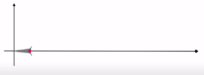
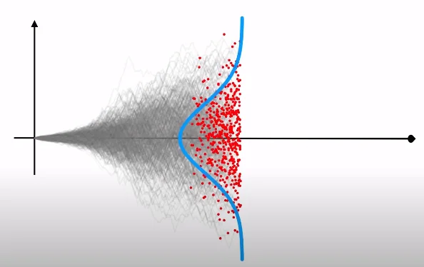
Essentially, over a short period of time, there’s not much influence on the stock price by random-walk steps to allow it to reach extreme deviations from the stock’s current price. But over a period of time, the probability of it reaching more extreme prices increases, but the majority of the expected stock price is still close to the stock’s current price. This may not be very consistent with our observation of the general trend of the market to increase over a long period of time, but back then, there wasn’t a lot of data available and this is how Bachelier modeled it. So after a short time, the stock price could only move up or down a little, but after more time, a wider range of prices is possible. He modeled the expected future price of a stock by a normal distribution, centered on the current price which spreads out over time.
Side note: He realized that he had rediscovered the exact equation which describes how head radiates from regions of high temperature to regions of low temperature, originally discovered by Joseph Fourier in 1822. Thus, he called his discovery the ‘radiation of probabilities’. Bachelier’s random walk theory would later find application in solving the longstanding physics mystery of Brownian motion, the erratic movement of microscopic particles observed by botanist Robert Brown. Remarkably, Albert Einstein, in his explanation of Brownian motion in 1905, unknowingly built upon the same random walk principles established by Bachelier years earlier.
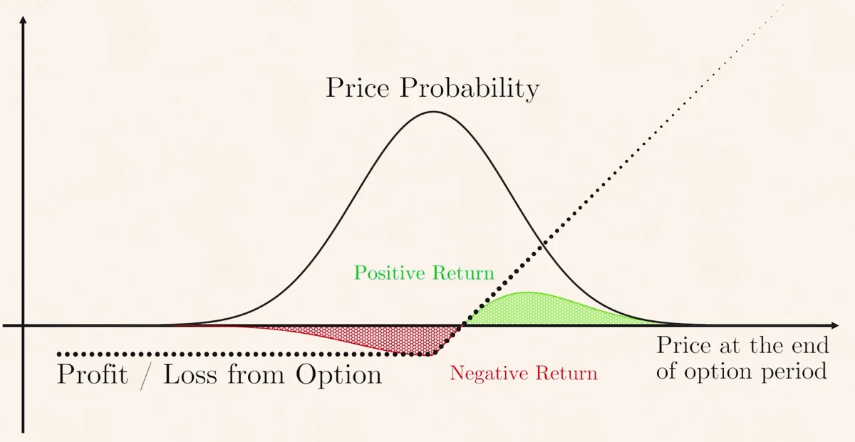
Bachelier’s crowing achievement, was that he had finally figured out a mathematical way to price an option by applying his random walk theory.
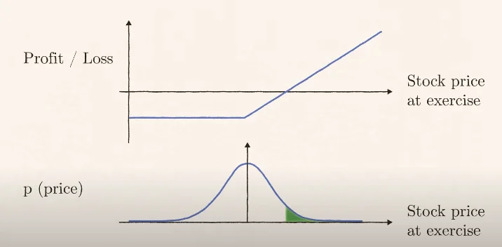
- The probability that the option buyer makes profit is the probability that the stock price increases by more than the price paid for the option. We call this the stock price at exercise. Otherwise the buyer would just let the option expire. This is the green shaded area.
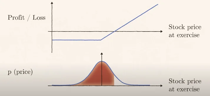
- The probability that the option seller makes profit is the probability that the stock price stays low enough that the buyer doesn’t earn more than they paid for it. Note that this is sufficient, because even if the stock price has increased from the strike price, but not by enough to increase past an amount that allows the buyer to exercise the option, the premium payed for by the buyer is enough to give the seller more profit than what would be obtained if he didn’t sell the option. This is the red shaded area.
Note that you can influence the region of probabilities simply by changing the premium (price) of the option. Increase the premium, and the stock price required for the option buyer to exercise the option increases. Pushing the probability region where he makes a profit further toward the edges. You can calculate the expected return of buying / selling an option simply by multiplying the profit / loss each individual stands to gain / lose by the probability of each outcome. Note that each probability here is just a function of the price of the option. Bachelier argued that a fair price for an option is what makes the expected return for buyers and sellers equal.
When Bachelier finished his thesis, he had beaten Einstein to inventing the random walk and solved the problem that had eluded options traders for hundreds of years. But no one noticed. The physicists were uninterested and traders weren’t ready. The key thing missing was a way to make a ton of money.
The Bachelier Model
What Bachelier essentially gave us, was a closed form equation for pricing a call / put option under the Bachelier model. The Bachelier model is basically representing a forward price contract (process) as a stochastic differential equation. Here, $\sigma$ is volatility.
$$dF_t = \sigma dW_t, \ t \in [0, T]$$You can think of $[0, T]$ as sort of representing a single time-step. Although this is a continuous process, we can think of it as a discrete process where we’re using very small values for the time-step $(T = dt)$. Solving for the forward price process, we get:
$$ \begin{align} & \int_0^TdF_t = \int_0^T\sigma dW_t \\ \\ & F_t - F_0 = \sigma(W_t-W_0) \quad | \ W_0 \text{ is 0 by the definition of brownian motion} \\ \\ & F_T = F_0 + \sigma W_t \end{align} $$And that’s it. An elegant way to model the future price and derive the closed form for pricing options. More generally, we can write the above result as $F_{t+1} = F_t + \sigma W_t$. We can even prove that $F_t$ is a martingale. That is:
$$ \mathbb{E}[F_{t+1}|F_t] = F_t $$It’s essentially saying that the forward price process at some point in the future is expected to be $F_t$. Our best guess for the next step in the process, is just the latest point computed in the process. Proof:
$$ \mathbb{E}[F_{t+1}|F_t] = \mathbb{E}[F_t + \sigma W_{t+1}|F_t] = \mathbb{E}[F_t + \sigma W_{t+1}] = F_t $$Pricing a Call Option
We are going to be pricing European style options, that is, we will be considering the payoff at maturity, at time $T$. We don’t know what the future holds for the derivative, but we know what the value of that derivative could be at some time $T$ in the future. Essentially, based on the price of the underlying asset that the derivative is tracking at expiration, we know that the payoff is going to take the shape of a hockey-stick figure as shown previously. A call option at time $T$, will give us:
$$ \begin{align*} & K \text{ - Strike Price} \\ & T \text{ - Time to Maturity} \\ & C_T = max((F_t-K), 0)=(F_T - K)^+ \end{align*} $$We use the $(\cdots)^+$ notation just to simplify the expression. At time $T$, this is a deterministic expression to how much payoff we make. But the issue is we do not know what $F_T$ will be. So the best thing to do today would be to compute the expectation of that payoff and hope to derive a closed form equation to compute the call price. The call price today is given by the expectation of the future:
$$ \begin{align*} & C_0 = \mathbb{E}[(F_T - K)^+] \\ & = \mathbb{E}[(F_0 + \sigma W_T - K)^*] \end{align*} $$Now, $W_T$ is still an increment in Brownian motion, that is, it is distributed normally with a mean of 0 and a variance of $dt$. Note $dt = T$. And since variance is equivalent to the square of the standard deviation, we can write the equation as:
$$ = \mathbb{E}[(F_0 - \sigma \sqrt{(T - 0)}Z - K)^+] $$Where $Z \sim N(0, 1)$, $Z$ is a standard normal random variable. Essentially, we use the fact that we have independent stationary increments with mean 0 and variance $dt$ to substitute for $W_T$. Let’s rearrange some terms to get:
$$ = \mathbb{E}[(F_0 - K - \sigma\sqrt{T}Z)^+] $$We want some more algebraic / better mathematical tools to substitute for the $max$ function. We will use indicators to make this equation easier to solve. Recall that:
$$ \mathbb{1}(x) = \begin{cases} 1 & \text{condition of } x\\ 0 & \sim \text{condition of } x\\ \end{cases} $$The $max$ function in this context essentially just implies that when exercising an option, if there is positive payoff, take it, otherwise don’t take it (let it expire). And the indicator function let’s us imply the same thing in the equation. So we can substitute the indicator function in for the $max$ function be defining our indicator $\mathbb{1}$ as follows:
$$ \mathbb{1}(Z) = \begin{cases} 1 & Z \leq \frac{F_0 - K}{\sigma \sqrt T} \\ 0 & Z \gt \frac{F_0 - K}{\sigma \sqrt T} \\ \end{cases} $$Substituting this in:
$$ = \mathbb{E}[((F_0 - K - \sigma\sqrt TZ))\mathbb{1}_{Z \leq\frac{F_0-K}{\sigma\sqrt T}}] $$Distributing the indicator function yields:
$$ = \mathbb{E}[(F_0 - K)\mathbb{1}_{Z \leq\frac{F_0-K}{\sigma\sqrt T}} - \sigma \sqrt TZ\mathbb{1}_{Z \leq\frac{F_0-K}{\sigma\sqrt T}}] $$Now, since we know that $Z$ is distributed standard normally, the expectation that $Z$ is less than some quantity can be found by using the cumulative distribution function for the normal distribution. Essentially, the first term indicator function can be replaced by just substituting it with the normal cumulative distribution, $\Phi$, up to the indicator function value:
$$ = (F_0 - K) \Phi(\frac{F_0 - K}{\sigma \sqrt T}) - \sigma \sqrt T \mathbb{E}[Z\mathbb{1}_{Z \leq \frac{F_0 - K}{\sigma \sqrt T}}] $$Using properties of normal distributions, the derivative of the CDF $\Phi'(x) = -x\phi(x)$, where $\phi$ is the probability density function of the normal distribution.
$$ \phi(x) = \frac{1}{\sqrt{2\pi}}e^{\frac{-x^2}{2}} $$We can use this property to solve the second term since:
$$ \mathbb{E}[Z\mathbb{1}_{Z \leq y}] = \int_{-\infty}^y x\phi(x)dx = -\phi(y) $$Applying this to the original equation by letting $y = \frac{F_0 - K}{\sigma \sqrt T}$, we get:
$$ C_0 = (F_0 - K)\Phi(\frac{F_0 - K}{\sigma \sqrt T}) + \sigma\sqrt T\phi(\frac{F_0 - K}{\sigma \sqrt T}) $$A closed form equation for pricing a call option given the current asset price $F_0$, the strike price $K$, the volatility $\sigma$ and the time to maturity $T$ of the option!
We can similarly use the Bachelier model to price all other kinds of future contracts, including put options, call / put futures, etc.
Phase 1.5 - Brownian Motion $B_t$ (Wiener Process)
So Brown discovered that any particles, if they were small enough, exhibited this random movement, which came to be known as Brownian motion. But what caused it remained a mystery. 80 years later in 1905, Einstein figured out the answer. Over the previous couple hundred years, the idea that gases and liquids were made up of molecules became more and more popular. But not everyone was convinced that molecules were real in a physical sense. Just that the theory explained a lot of observations. The idea led Einstein to hypothesize that Brownian motion is caused by the trillions of molecules hitting the particle from every direction, every instant. Occasionally, more will hit from one side than the other, and the particle will momentarily jump. To derive the mathematics, Einstein supposed that as an observer we can’t see or predict these collisions with any certainty. So at any time we have to assume that the particle is just as likely to move in one direction as an another. So just like stock prices, microscopic particles move like a ball falling down a galton board, the expected location of a particle is described by a normal distribution, which broadens with time. It’s why even in completely still water, microscopic particles spread out. This is diffusion. By solving the Brownian motion mystery. Einstein had found definitive evidence that atoms and molecules exist. Of course, he had no idea that Bachelier had uncovered the random walk five years earlier. - The Trillion Dollar Equation
The random walk that Bachelier came up with and the Brownian motion that Robert Brown discovered are both pretty similar and following the developments that occurred in mathematically developing Brownian motion will help us understand more complex future contracts pricing models.
Definition: A standard (one-dimensional) Brownian Motion (also called Wiener Process) is a stochastic process $\{W_t\}_{t \geq 0+}$ indexed by non-negative real numbers $t$ with the following properties:
- $W_0 = 0$.
- With probability 1, the function $t \to W_t$ is continuous in $t$.
- The process $\{W_t\}_{t \geq 0+}$ has stationary, independent increments.
- The increment $W_{t+s} - W_s$ has the $\text{NORMAL}(0, t)$ distribution
I’ll explain these properties in more details below. Let’s call them the axioms that govern all Wiener processes / Brownian motion.
Axioms
Brownian Motion has independent increments. Say we have a time value $r$, $s$ and $t$. We have some Brownian motion associated with each of these time values. The time from $s \to t$ is an increment. So is the time from $r \to s$. We’re essentially saying that the increment from $s \to t$ is totally independent of other time periods, not even the previous $r \to s$ time period. In short, this axiom essentially says that whatever happens in any given time period is totally random and does not depend on what happens in any other time period.
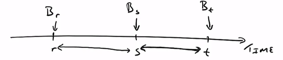
Brownian Motion has stationary increments. It’s sort of related to the previous axiom. But what it essentially says that the distirbution in the time between $s \to t$ only depends on the time values $t$ and $s$ and nothing else.
Brownian Motion has Normal Distribution. If we look at the distribution in any time-step, the data points will be normally distributed. That is:
$$ B_t - B_s \sim N(\mu(t - s), \sigma^2(t-s)) $$Here, the term $\mu (t-s)$ is the mean of the normal distribution. This term is also often called drift. The $\sigma^2(t-s)$ term is the variance of the normal distribution. $\sigma$ is just the standard deviation.
Brownian Motion has continuous sample paths. This simply just means that at any time value, the Brownian motion graph is continuous at all points.
Standard Brownian Motion
Standard Brownian Motion is a specialized case of Brownian Motion. It is the case that Bachelier studied and used to model future stock prices in his PhD Thesis. Here, Brownian motion has a standard normal distribution. A standard normal distribution has mean $(\mu) = 0$ and variance $\sigma^2 = 1$.
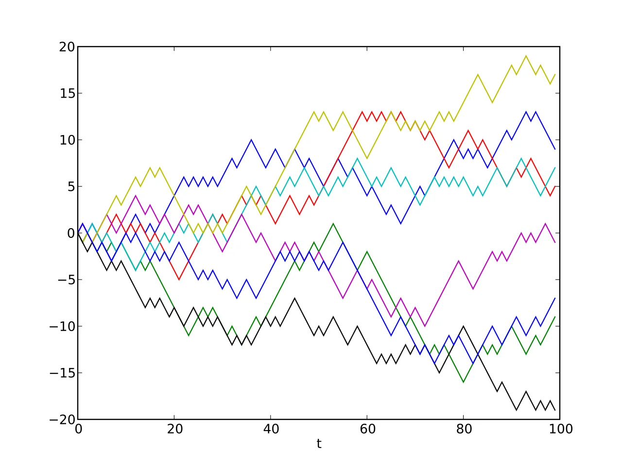
Random Walks
A symmetric random walk is a mathematical model that describes a path consisting of a series of random steps, where each step has an equal probability of being taken in either direction. We will limit our discussion to symmetric random walks. Here symmetric just means that the probability of each step being chosen is equal.
Let $S_n$ denote the position of the walker after $n$ steps. Then, a symmetric random walk can be defined recursively as:
$$ X_n = X_{n-1} + Z_n$$Here, $Z_n$ are independent and identically distributed random variables taking values $+1$ or $-1$ with equal probability, i.e., $P(Z_n = 1) = P(Z_n = -1) = \frac{1}{2}$.
Effectively, when we consider the discrete case, we call it a random walk. But as we keep reducing our time-steps, that is, $\Delta t \to 0$, it’s the same as Brownian motion. The summation formula is the mean by definition, so we can write $Z_k = \pm\frac{t}{n}$, where $n$ is the number of time steps. For convenience, let us write $Z_k = \pm \sqrt \frac{t}{n}$.
Expectation
The expectation of $Z_k$, $\mathbb{E}[Z_k] = 0 \iff \mathbb{E}[X_n] = 0$. The expectation, $\mathbb{E}[Z_k^2] = \frac{t}{n}$. Now when working with expected values, due to LINEARITY OF EXPECTATION, $\mathbb{E}[Z_i Z_j] = \mathbb{E}[Z_i] \cdot \mathbb{E}[Z_j] = 0$ .
$$ \begin{align} & \mathbb{E}[X_n^2] = \mathbb{E}[(\sum Z_k)^2] \\ & = \mathbb{E}[(Z_1 + Z_2 + \cdots + Z_n)(Z_1 + Z_2 + \cdots + Z_n)] \\ & = \mathbb{E}[Z_1^2 + Z_1Z_2 + \cdots + Z_1Z_n + Z_2Z_1 + \cdots + Z_2Z_n + \cdots + Z_nZ_1 + Z_nZ_2+\cdots+Z_n^2] \ | \text{Since } \mathbb{E}[Z_iZ_j] = 0 \text{ for } i \neq j \\ & = \mathbb{E}[\sum Z_k^2] \\ & = \mathbb{E}[Z_1^2] + \mathbb{E}[Z_2^2] + \cdots + \mathbb{E}[Z_n^2] \\ & = \frac{t}{n} + \frac{t}{n} + \cdots + \frac{t}{n} \\ & \implies \mathbb{E}[X_n^2] = t \end{align} $$The important property here is that this expectation is completely independent of $n$. No matter how many time steps we take, the expectation is just $t$. To go from the discrete case to the continuous case, we can indicate the size of time-steps going to 0 as $n \to \infty$. Because $\mathbb{E}[X_n] = 0$ and $\mathbb{E}[X_n^2] = t$ (both are independent of $n$), we know that the exact same expectations apply to the Brownian Motion case as well. As $n \to \infty$, our random walk becomes Brownian Motion. Therefore, we get:
$$ \begin{align} & \mathbb{E}[B_t] = 0 \\ & \mathbb{E}[B_t^2] = t \end{align} $$- Brownian Motion is bounded. This just says that, in the context of share prices, a share price cannot go to $\infty$.
- Brownian Motion is a Markov process. This follows from the definition.
- Brownian Motion is a Martingale. This is sort of like saying, the best guess for what happens next (in the future), is what’s happening now. More formally, $\mathbb{E}[Z_{t+1}|Z_t] = Z_t$. Kind of paradoxical.
Geometric Brownian Motion
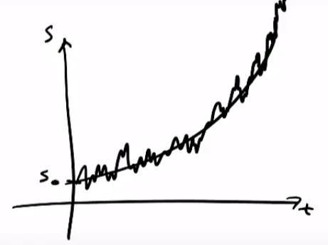
Remember that in Bachelier’s Thesis, he modeled share prices using a standard normal distribution. But looking at share prices almost immediately indicates an issue with his model. We notice that over time, stocks tend to drift in one direction or the other, with total markets having an overall upwards drift. This is sort of like having the normal distribution have it’s mean drifted up from 0. This is the idea that we want to model using geometric Brownian motion.
We sort of expect share prices to grow in an exponential manner. We mathematically write this as $S_t = S_0e^{\alpha t}$. Just the formula to denote standard exponential growth. But we know that share prices follow Brownian motion (random walk), and the price keeps constantly fluctuating. Effectively, we need to introduce a parameter in this equation to account for the Brownian motion. So to take this into account, we can do this by modifying the model slightly to $S_t = S_0 e^{\alpha t + \beta B_t}$. The term $\beta B_t$ accounts for the Brownian motion. $\beta$ is a constant, which is very difficult to measure for a stock. The term is essentially supposed to be a measure of volatility. You can see that with higher $\beta$, you have more contribution from the Brownian motion term and hence have more random volatility.
If we play around with the formula a bit, we can do the following:
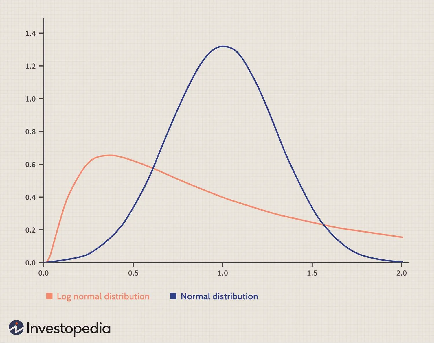
$$ \begin{align} & \frac{S_t}{S_0} = e^{\alpha t + \beta B_t} \\ & \ln(\frac{S_t}{S_0}) = \alpha t + \beta B_t \quad \text{You can think of the } \alpha t \text{ term as contributing to the mean and } \beta B_t \text{ as a normal distribution with mean } 0\\ & \text{Since, } B_t \sim N(0, t) \\ & \alpha t + \beta B_t \text{ is normally distributed, but we want to know it's mean and variance} \\ & \alpha t + \beta B_t \sim N(\alpha t, \beta^2t) \quad | \text{ Since } Var(x) = a \implies Var(kx) = k^2a\\ & \implies \ln(\frac{S_t}{S_0}) \sim N(\alpha t, \beta^2 t) \end{align} $$This is what is known as log-normal. In other words, the ratio of the share prices at time $t$ to the share price at the beginning is a log-normal distribution. The log part essentially just skews the curve.
Phase 2 - The Black-Scholes-Merton Equation
Thorpe wasn’t satisfied with Bachelier’s model for pricing options. For one thing, stock prices aren’t entirely random. They can increase over time if the business is doing well or fall if it isn’t. Bachelier’s model ignores this. So Thorpe came up with a more accurate model for pricing options, which took this drift into account. He used his model to gain an edge in the market and make a lot of money. Black-Scholes and Merton later independently came up with a way to price future contracts that would then revolutionize the trading industry forever. Their equation, like Thorpe’s, was an improved version of Bachelier’s model.
Dynamic Hedging
A Toy Example
Let’s say Bharat sells Arya a call option on a stock, and let’s say the stock price has gone up. So it’s now in the money for Arya. For every additional rupee that the stock price goes up from the strike price, Bharat will now lose a rupee. BUT, he can eliminate this risk by owning 1 unit of stock. He would lose 1 rupee from the option, but gain that rupee back from the stock. And if the stock drops below the strike price, making the option go out of the money for Arya, he can just sell the stock at the strike price so he doesn’t risk losing any money from that either. This is the idea behind dynamic hedging.
A Hedged Portfolio
A hedged portfolio, at any one time, will offset an option $V$ with some amount ($\Delta$) of stock $S$. Let $\Pi$ represent the portfolio, we have $\Pi = V - \Delta S$. It basically means you can sell something without taking the opposite side of the trade. You have a no-risk trade you could make profit from. However, this isn’t very practical because the amount of stock to hold $\Delta$, changes based on current stock prices.
Deriving Black-Scholes-Merton
We’re essentially constructing a portfolio of a single option $V$, and a certain number of shares $\Delta$ of $S$ that we’re going to sell against the option to dynamically hedge against it. So the value of our portfolio is essentially $\Pi = V(S, t) - \Delta S$. We’re interested in tracking the time evolution of our portfolio. This is difficult because again, the future cash-flow of our option is not easy to price in. So we use the principles from Brownian motion to essentially model the underlying asset as a stochastic process that follows geometric Brownian motion.
Our portfolio is now just a $dt$ term which means that the portfolio is now deterministic, and as such, doesn’t carry any risk. A risk-free portfolio should yield a risk-free rate ($r$), which let’s us write a different equation for $d\Pi$.
$$ \begin{align} & d\Pi = r\Pi dt = (V - rS\frac{\partial V}{\partial S})dt \\ & \text{By equating this to our previous formula, and re-grouping terms, we get the famous equation:} \\ & \frac{\partial V}{\partial t} + rS\frac{\partial V}{\partial S} + \frac{1}{2}\sigma^2S^2\frac{\partial^2V}{\partial S^2}-rV = 0 \end{align} $$The risk-free rate in the Black-Scholes formula represents the theoretical return on an investment with no risk of default. For example, government-bonds.
We can now set $V$ equal to a call option or a put option and then solve the differential equation to get a closed-form equation for the price of a call-option given:
$$ \begin{align} & C = \text{call option price} \\ & N = \text{cumulative distribution function of the normal distribution} \\ & S_t = \text{spot price of an asset} \\ & K = \text{strike price} \\ & r = \text{risk-free rate} \\ & t = \text{time to maturity} \\ & \sigma = \text{volatility of asset} \\ & \\ & C = N(d_1)S_t - N(d_2)Ke^{-rt} \\ & \text{where } d_1 = \frac{\ln(\frac{S_t}{K}) + (r + \frac{\sigma^2}{2})t}{\sigma\sqrt t} \\ & \text{and } d_2 = d_1 - \sigma\sqrt t \end{align} $$