FFT (Fast Fourier Transform)

The problem: Given two d-degree polynomials, compute their product

Let $A(x) = a_0 + a_1x + ... + a_dx^d \ \text{and} \ B(x) = b_0 + b_1+...+b_dx^d$

Then,

$C(x) = A(x)\times B(x) = c_0 + c_1x+...+ c_{2d}x^{2d}$ has coefficients $c_k = a_ob_k+a_1b_{k-1}+...+a_kb_0 = \sum_{i=0}^ka_ib_{k-i}$

The naïve solution here would be to compute in $O(d^2)$ steps. There are $2d$ terms in the final expression and each of these terms requires order $O(d)$ multiplications to compute. The question is, can we do better?

Divide and conquer is an approach that works well when we are able to introduce/identify some sort of overlap in subproblems. But for each coefficient, the multiplication terms do not have much overlap. Perhaps a different view is of order.

The co-efficient representation of polynomials is essentially an equation that can uniquely identify some function on a graph. There are definitely other representations that will allow us to do the same.

The one we will be looking at today is the value representation of a function. Consider any function defined by some $d$ degree polynomial. Notice that such a function can always be uniquely identified by any set of $d+1$ points that satisfy the equation (are on its graph).

Proof: Say we have a $d$ degree polynomial $P$ and we evaluate it at $d + 1$ unique points. We end up with the set of points $\{ (x_0, P(x_0)), (x_1, P(x_1), \dots, (x_d, P(x_d) \}$.

If $P(x) = p_dx^d + p_{d-1}x^{d-1}+\dots+p_2x^2+p_1x^1+p_0$

Notice that there are $d+1$ coefficients for each such $P(x)$. Writing our equation in matrix form,

Notice that there are $d+1$ variables and $d+1$ equations. If we had any lesser we would not be able to uniquely solve for this system. Hence we need at least $d+1$ points. Another way to visualize this is that our matrix of equations is invertible for unique points $x_0, x_1, \dots, x_d$. This can be proved by solving for the determinant. This implies that we have a unique set of coefficients with which we can identify the polynomial.

But why do we care about the value representation of a polynomial?

Value representation: The good and the bad

Notice that if we have some polynomial $C(x)$ which is the result of multiplication of two $d$ degree polynomials $A(x)$ and $B(x)$, the degree of polynomial $C(x)$ must be $2d$. This means that it can be uniquely identified by just $2d+1$ points.

Now, for some point $x_0$, $C(x_0) = A(x_0)\times B(x_0)$.

This means that, if we could pick and evaluate polynomials $A(x)$ and $B(x)$ at $2d+1$ points, we can generate $2d+1$ points to uniquely identify $C(x_0)$ with in linear time.

However, this is assuming that converting the polynomial from coefficient form to value form and back takes lesser than equal to $O(n)$. This is not true. We must evaluate a polynomial with $d$ terms at $2d+1$ points. This calculation is of the order $O(d^2)$ and hence, no better than the naïve method. This is where the idea of FFTs comes in.

Evaluating faster (Applying divide and conquer)

The problem we wish to solve is as follows. Given a polynomial function $A(x)$ and a set of points $X$, we wish to compute $A(x) \ \ \forall x \in X$.

Let $A(x) = a_0+a_1x+\dots+a_dx^{n-1}$

Notice that we can divide our polynomial into two halves, one containing the even powers of $x$ and another containing the odd halves. Let’s call them $A_e(x)$ and $A_o(x)$.

$A_e(x) = \sum_{k=0}^{\frac{n}{2}-1}a_{2k}x^k$

$A_o(x) = \sum_{k=0}^{\frac{n}{2}}a_{2k+1}x^k$

Notice that we aren’t raising $x$ to the power of their coefficients. And in doing so, we have effectively cut in half the degree of the polynomial. But in doing so, we have lost the original polynomial. We still require an algebraically correct way to merge these two divisions into the original polynomial.

Notice that if we evaluate $A_e$ at $x^2$ instead of $x$, the algebra checks out. $(x^2)^k = x^{2k}$. Every polynomial term matches its counterpart in the original polynomial. Similarly, we can do the same for $A_0$, but we are now missing a $+1$ in the powers of every term. This can be easily corrected by simply multiplying a single $x$ to the whole polynomial. Similar to Horner’s rule. This gives us our final equation,

This has allowed us to effectively calculate the value of $A(x)$ for some point using a technique that uses divide and conquer. But is it truly faster than any of the previous algorithms?

Analyzing time complexity

Notice that

The $\frac{n}{2}$ comes from dividing the input to each recurrence in half. We have 2 such recursive calls. These 2 factors account for the first term in the expression. Now, at each “node” of our recursive tree, we have do $O(n)$ computation for traversing the polynomial list and splitting it into two halves. And finally, $O(|X|)$ time for computing the polynomial at each $x\in X$.

To solve this recurrence, let us imagine the recursion tree. The base case for this recursion is when $n=1$. When $n=1$, the answer is the value in the set itself. However, notice that at no point are we ever changing the size of the set $X$. The original size of $X$ was $n$, and it remains $n$ at every step of the algorithm. This will span out to be a binary tree of depth $log_2(n)$, with each node doing $O(n)$ computation.

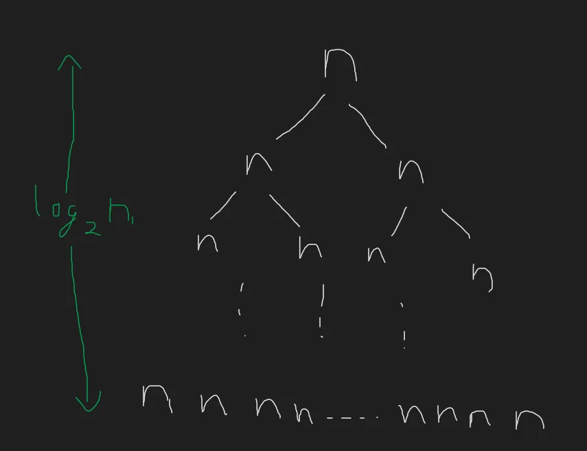
At the bottom most level, notice that we still have order $n$ leaves, each of which are doing order $n$ computation. This will sadly give us a time complexity of $O(n \times n) = O(n^2)$.

The reason why every node must do $O(n)$ computation is because we haven’t been able to change the size of the set $X$ like we have managed to with $n$. If we could somehow half the size of $X$ just like we did with $n$, we would get a much simpler recurrence. $T(n) = T(\frac{n}{2})+O(n)$ which evaluates to just $O(nlogn)$. But how can we reduce the size of the set of all points we need to evaluate our polynomial at?

The final piece of the puzzle

Let’s take a look at our equation again

In the recursive call to $A_e$ and $A_o$, we have so far managed to reduce the value of $n$ (no. of terms in the polynomial), by half. But we haven’t managed to half the size of $X$, the set of all points we require to evaluate our polynomial at. So let’s take our attention off $n$ and think about $x$.

At every step, or “node” of our algorithm, notice that we are passing the value of $x^2$. Another key realization is that, we are free to choose any $X$ we want as long as all the points in $X$ are unique.

This has allowed us to transform the problem of reducing the size of $X$ into a simpler question, “Does there exist some $x^2$ for which there are multiple unique roots $x_0$ and $x_1$?”

Notice that at least in the real plane, the answer is no. Well, it might work for the first “root node” of our recursion tree. Every real number except zero satisfies the property that $x^2=(-x)^2$. Hence we can just evaluate the polynomial at some set of points $x$ and $-x$. But in the second level of our recursion, we have a huge problem. $x^2$ will always be a positive value. This means, we no longer have positive-negative pairs to work with. Our set $X$ is no longer free to choose. It has the constraint on it that it must be all positive. Without our $\pm x$ pairs, we cannot proceed.

Breaking out of the real plane

Here comes the last piece of our puzzle. While the above was true for real numbers, it is not true for complex numbers. Let’s assume our set at the final depth of its recursion was $X = \{ 1 \}$.

For the set to be halved in the level just above, we require two values of $x_0$ and $x_1$ such that $x_0^2=x_1^2=1$.

Two such values are $-1$ and $+1$. Let’s try thinking one level above this. We would require two values $x_0$ and $x_1$ such that $x_0^2=x_1^2=-1$. Two values that fit this equation are $i$ and $-i$.

Notice that we can keep doing this at every step of our recursion, and we would just keep picking the $k^{th}$ roots of $1$ and every level.

This is the key realization to solving the problem of reducing the size of $X$. By choosing our set $X$ as the set of all the $k^{th}$ roots of unity where $k \gt log_2n$, we have effectively managed to half the size of $X$ along with $n$ at every step of our algorithm. Our recursion tree now looks more like this

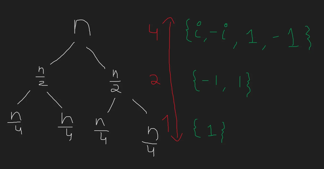
By simply computing $A_e(x)$ and $A_o(x)$ at $\frac{n}{2}$ intervals, we can compute the answer at $n$ points. The roots of unity always occur in $\pm$ pairs and evaluate to the same value when squared. This means, we can write it as follows.

This has allowed us to transform our original equation for calculating time complexity into he following

We have managed to come up with an algorithm that can compute the value of some polynomial function $A(x)$ with $n$ terms at every point in some set $X$ of size of the order $n$ in $O(nlogn)$ time.

Converting back to polynomial form [Interpolation]

Now, we have an algorithm that can almost do it all. We can compute form polynomial representation to value representation in just $O(nlogn)$ complexity. We can compute the value of the product of the $2n$ terms and find the value representation of the polynomial product in $O(n)$ complexity. The only thing left is to convert the polynomial obtained back from value form to polynomial form.

With a little thought, we can use the same FFT algorithm we just came up with to interpolate our values back to give us our polynomial in coefficient form. Let us think about the original equation that we managed to simplify and solve using FFT.

We chose a value of $x_i$ such that every $x_i \in X$, is some $k^{th}$ root of unity. To get our original vector back, we only need to left-multiply the matrix of the $k^{th}$ roots of unity with it’s inverse and use FFT to compute the product of the inverse matrix and the values vector.

This was our choice for the $X$ matrix,

$M_n(\omega)$ is a Vandermonde matrix with the following property that it is invertible only if every choice of $x_i$ is unique. This is true in our case and hence $M_n(\omega)$ is invertible. Once this proof has been done for the sake of proving correctness, we have a complete solution to solve the problem of polynomial multiplication in just $O(nlogn)$ time.

The overall time complexity is $O(nlogn)+O(n)+O(nlogn) = O(nlogn)$

References

These notes are old and I did not rigorously horde references back then. If some part of this content is your’s or you know where it’s from then do reach out to me and I’ll update it.

1. Professor Kannan Srinathan’s course on Algorithm Analysis & Design in IIIT-H
2. Divide & Conquer: FFT - MIT 6.046J OCW - Erik Demaine